3.2.2 Axis and ticks 
MathGL library can draw not only the bounding box but also the axes, grids, labels and so on. The ranges of axes and their origin (the point of intersection) are determined by functions SetRange(), SetRanges(), SetOrigin() (see Ranges (bounding box)). Ticks on axis are specified by function SetTicks, SetTicksVal, SetTicksTime (see Ticks). But usually
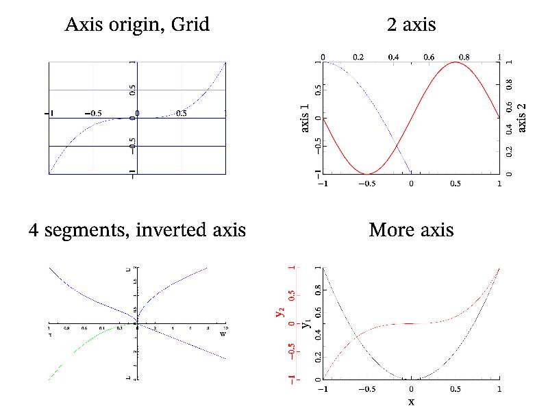
Function axis draws axes. Its textual string shows in which directions the axis or axes will be drawn (by default "xyz", function draws axes in all directions). Function grid draws grid perpendicularly to specified directions. Example of axes and grid drawing is:
int sample(mglGraph *gr)
{
  gr->SubPlot(2,2,0); gr->Title("Axis origin, Grid"); gr->SetOrigin(0,0);
  gr->Axis(); gr->Grid(); gr->FPlot("x^3");

  gr->SubPlot(2,2,1); gr->Title("2 axis");
  gr->SetRanges(-1,1,-1,1); gr->SetOrigin(-1,-1,-1);  // first axis
  gr->Axis(); gr->Label('y',"axis 1",0);  gr->FPlot("sin(pi*x)");
  gr->SetRanges(0,1,0,1);   gr->SetOrigin(1,1,1);   // second axis
  gr->Axis(); gr->Label('y',"axis 2",0);  gr->FPlot("cos(pi*x)");

  gr->SubPlot(2,2,3); gr->Title("More axis");
  gr->SetOrigin(NAN,NAN); gr->SetRange('x',-1,1);
  gr->Axis(); gr->Label('x',"x",0); gr->Label('y',"y_1",0);
  gr->FPlot("x^2","k");
  gr->SetRanges(-1,1,-1,1); gr->SetOrigin(-1.3,-1); // second axis
  gr->Axis("y","r");  gr->Label('y',"#r{y_2}",0.2);
  gr->FPlot("x^3","r");

  gr->SubPlot(2,2,2); gr->Title("4 segments, inverted axis");
  gr->SetOrigin(0,0);
  gr->InPlot(0.5,1,0.5,1);  gr->SetRanges(0,10,0,2);  gr->Axis();
  gr->FPlot("sqrt(x/2)");   gr->Label('x',"W",1); gr->Label('y',"U",1);
  gr->InPlot(0,0.5,0.5,1);  gr->SetRanges(1,0,0,2); gr->Axis("x");
  gr->FPlot("sqrt(x)+x^3"); gr->Label('x',"\\tau",-1);
  gr->InPlot(0.5,1,0,0.5);  gr->SetRanges(0,10,4,0);  gr->Axis("y");
  gr->FPlot("x/4"); gr->Label('y',"L",-1);
  gr->InPlot(0,0.5,0,0.5);  gr->SetRanges(1,0,4,0); gr->FPlot("4*x^2");
  return 0;
}
Note, that MathGL can draw not only single axis (which is default). But also several axis on the plot (see right plots). The idea is that the change of settings does not influence on the already drawn graphics. So, for 2-axes I setup the first axis and draw everything concerning it. Then I setup the second axis and draw things for the second axis. Generally, the similar idea allows one to draw rather complicated plot of 4 axis with different ranges (see bottom left plot).
At this inverted axis can be created by 2 methods. First one is used in this sample – just specify minimal axis value to be large than maximal one. This method work well for 2D axis, but can wrongly place labels in 3D case. Second method is more general and work in 3D case too – just use aspect function with negative arguments. For example, following code will produce exactly the same result for 2D case, but 2nd variant will look better in 3D.
// variant 1
gr->SetRanges(0,10,4,0);  gr->Axis();

// variant 2
gr->SetRanges(0,10,0,4);  gr->Aspect(1,-1);   gr->Axis();
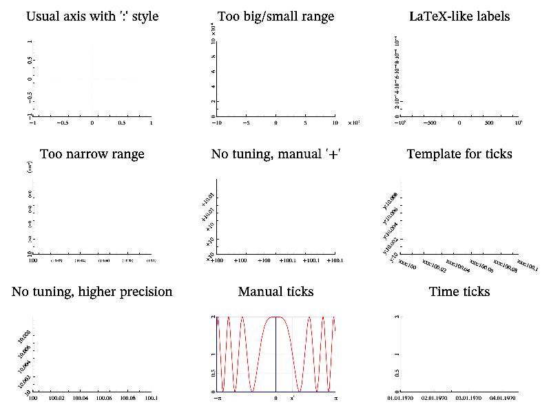
Another MathGL feature is fine ticks tunning. By default (if it is not changed by SetTicks function), MathGL try to adjust ticks positioning, so that they looks most human readable. At this, MathGL try to extract common factor for too large or too small axis ranges, as well as for too narrow ranges. Last one is non-common notation and can be disabled by SetTuneTicks function.
Also, one can specify its own ticks with arbitrary labels by help of SetTicksVal function. Or one can set ticks in time format. In last case MathGL will try to select optimal format for labels with automatic switching between years, months/days, hours/minutes/seconds or microseconds. However, you can specify its own time representation using formats described in http://www.manpagez.com/man/3/strftime/. Most common variants are ‘%X’ for national representation of time, ‘%x’ for national representation of date, ‘%Y’ for year with century.
The sample code, demonstrated ticks feature is
int sample(mglGraph *gr)
{
  gr->SubPlot(3,3,0); gr->Title("Usual axis");  gr->Axis();
  gr->SubPlot(3,3,1); gr->Title("Too big/small range");
  gr->SetRanges(-1000,1000,0,0.001);  gr->Axis();
  gr->SubPlot(3,3,2); gr->Title("LaTeX-like labels");
  gr->Axis("F!");
  gr->SubPlot(3,3,3); gr->Title("Too narrow range");
  gr->SetRanges(100,100.1,10,10.01);  gr->Axis();
  gr->SubPlot(3,3,4); gr->Title("No tuning, manual '+'");
  // for version<2.3 you need first call gr->SetTuneTicks(0);
  gr->Axis("+!");
  gr->SubPlot(3,3,5); gr->Title("Template for ticks");
  gr->SetTickTempl('x',"xxx:%g"); gr->SetTickTempl('y',"y:%g");
  gr->Axis();
  // now switch it off for other plots
  gr->SetTickTempl('x',"");   gr->SetTickTempl('y',"");
  gr->SubPlot(3,3,6); gr->Title("No tuning, higher precision");
  gr->Axis("!4");
  gr->SubPlot(3,3,7); gr->Title("Manual ticks");  gr->SetRanges(-M_PI,M_PI, 0, 2);
  gr->SetTicks('x',M_PI,0,0,"\\pi");  gr->AddTick('x',0.886,"x^*");
  // alternatively you can use following lines
  //double val[]={-M_PI, -M_PI/2, 0, 0.886, M_PI/2, M_PI};
  //gr->SetTicksVal('x', mglData(6,val), "-\\pi\n-\\pi/2\n0\nx^*\n\\pi/2\n\\pi");
  gr->Axis();  gr->Grid();  gr->FPlot("2*cos(x^2)^2", "r2");
  gr->SubPlot(3,3,8); gr->Title("Time ticks");  gr->SetRange('x',0,3e5);
  gr->SetTicksTime('x',0);  gr->Axis();
}
The last sample I want to show in this subsection is Log-axis. From MathGL’s point of view, the log-axis is particular case of general curvilinear coordinates. So, we need first define new coordinates (see also Curvilinear coordinates) by help of SetFunc or SetCoor functions. At this one should wary about proper axis range. So the code looks as following:
int sample(mglGraph *gr)
{
  gr->SubPlot(2,2,0,"<_");  gr->Title("Semi-log axis");
  gr->SetRanges(0.01,100,-1,1); gr->SetFunc("lg(x)","");
  gr->Axis(); gr->Grid("xy","g"); gr->FPlot("sin(1/x)");
  gr->Label('x',"x",0); gr->Label('y', "y = sin 1/x",0);

  gr->SubPlot(2,2,1,"<_");  gr->Title("Log-log axis");
  gr->SetRanges(0.01,100,0.1,100);  gr->SetFunc("lg(x)","lg(y)");
  gr->Axis(); gr->Grid("!","h=");   gr->Grid();
  gr->FPlot("sqrt(1+x^2)"); gr->Label('x',"x",0);
  gr->Label('y', "y = \\sqrt{1+x^2}",0);

  gr->SubPlot(2,2,2,"<_");  gr->Title("Minus-log axis");
  gr->SetRanges(-100,-0.01,-100,-0.1);  gr->SetFunc("-lg(-x)","-lg(-y)");
  gr->Axis(); gr->FPlot("-sqrt(1+x^2)");
  gr->Label('x',"x",0); gr->Label('y', "y = -\\sqrt{1+x^2}",0);

  gr->SubPlot(2,2,3,"<_");  gr->Title("Log-ticks");
  gr->SetRanges(0.1,100,0,100); gr->SetFunc("sqrt(x)","");
  gr->Axis(); gr->FPlot("x");
  gr->Label('x',"x",1); gr->Label('y', "y = x",0);
  return 0;
}
You can see that MathGL automatically switch to log-ticks as we define log-axis formula (in difference from v.1.*). Moreover, it switch to log-ticks for any formula if axis range will be large enough (see right bottom plot). Another interesting feature is that you not necessary define usual log-axis (i.e. when coordinates are positive), but you can define “minus-log” axis when coordinate is negative (see left bottom plot).


