---

3.3.3 Change data ¶

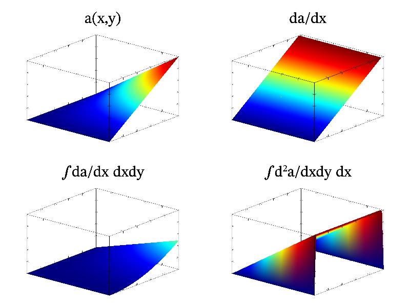
MathGL has functions for data processing: differentiating, integrating, smoothing and so on (for more detail, see Обработка данных). Let us consider some examples. The simplest ones are integration and differentiation. The direction in which operation will be performed is specified by textual string, which may contain symbols ‘x’, ‘y’ or ‘z’. For example, the call of Diff("x") will differentiate data along ‘x’ direction; the call of Integral("xy") perform the double integration of data along ‘x’ and ‘y’ directions; the call of Diff2("xyz") will apply 3d Laplace operator to data and so on. Example of this operations on 2d array a=x*y is presented in code:

int sample(mglGraph *gr)
{
  gr->SetRanges(0,1,0,1,0,1);
  mglData a(30,40); a.Modify("x*y");
  gr->SubPlot(2,2,0); gr->Rotate(60,40);
  gr->Surf(a);    gr->Box();
  gr->Puts(mglPoint(0.7,1,1.2),"a(x,y)");
  gr->SubPlot(2,2,1); gr->Rotate(60,40);
  a.Diff("x");    gr->Surf(a);  gr->Box();
  gr->Puts(mglPoint(0.7,1,1.2),"da/dx");
  gr->SubPlot(2,2,2); gr->Rotate(60,40);
  a.Integral("xy"); gr->Surf(a);  gr->Box();
  gr->Puts(mglPoint(0.7,1,1.2),"\\int da/dx dxdy");
  gr->SubPlot(2,2,3); gr->Rotate(60,40);
  a.Diff2("y"); gr->Surf(a);  gr->Box();
  gr->Puts(mglPoint(0.7,1,1.2),"\\int {d^2}a/dxdy dx");
  return 0;
}

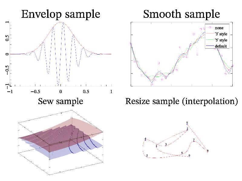
Data smoothing (function smooth) is more interesting and important. This function has single argument which define type of smoothing and its direction. Now 3 methods are supported: ‘3’ – linear averaging by 3 points, ‘5’ – linear averaging by 5 points, and default one – quadratic averaging by 5 points.

MathGL also have some amazing functions which is not so important for data processing as useful for data plotting. There are functions for finding envelope (useful for plotting rapidly oscillating data), for data sewing (useful to removing jumps on the phase), for data resizing (interpolation). Let me demonstrate it:

int sample(mglGraph *gr)
{
  gr->SubPlot(2,2,0,"");  gr->Title("Envelop sample");
  mglData d1(1000); gr->Fill(d1,"exp(-8*x^2)*sin(10*pi*x)");
  gr->Axis();     gr->Plot(d1, "b");
  d1.Envelop('x');  gr->Plot(d1, "r");

  gr->SubPlot(2,2,1,"");  gr->Title("Smooth sample");
  mglData y0(30),y1,y2,y3;
  gr->SetRanges(0,1,0,1);
  gr->Fill(y0, "0.4*sin(pi*x) + 0.3*cos(1.5*pi*x) - 0.4*sin(2*pi*x)+0.5*rnd");

  y1=y0;  y1.Smooth("x3");
  y2=y0;  y2.Smooth("x5");
  y3=y0;  y3.Smooth("x");

  gr->Plot(y0,"{m7}:s", "legend 'none'"); //gr->AddLegend("none","k");
  gr->Plot(y1,"r", "legend ''3' style'");
  gr->Plot(y2,"g", "legend ''5' style'");
  gr->Plot(y3,"b", "legend 'default'");
  gr->Legend();   gr->Box();

  gr->SubPlot(2,2,2);   gr->Title("Sew sample");
  mglData d2(100, 100); gr->Fill(d2, "mod((y^2-(1-x)^2)/2,0.1)");
  gr->Rotate(50, 60);   gr->Light(true);  gr->Alpha(true);
  gr->Box();            gr->Surf(d2, "b");
  d2.Sew("xy", 0.1);  gr->Surf(d2, "r");

  gr->SubPlot(2,2,3);   gr->Title("Resize sample (interpolation)");
  mglData x0(10), v0(10), x1, v1;
  gr->Fill(x0,"rnd");     gr->Fill(v0,"rnd");
  x1 = x0.Resize(100);    v1 = v0.Resize(100);
  gr->Plot(x0,v0,"b+ ");  gr->Plot(x1,v1,"r-");
  gr->Label(x0,v0,"%n");
  return 0;
}

Also one can create new data arrays on base of the existing one: extract slice, row or column of data (subdata), summarize along a direction(s) (sum), find distribution of data elements (hist) and so on.

Another interesting feature of MathGL is interpolation and root-finding. There are several functions for linear and cubic spline interpolation (see Интерполяция). Also there is a function evaluate which do interpolation of data array for values of each data element of index data. It look as indirect access to the data elements.

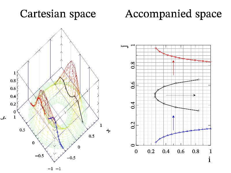
This function have inverse function solve which find array of indexes at which data array is equal to given value (i.e. work as root finding). But solve function have the issue – usually multidimensional data (2d and 3d ones) have an infinite number of indexes which give some value. This is contour lines for 2d data, or isosurface(s) for 3d data. So, solve function will return index only in given direction, assuming that other index(es) are the same as equidistant index(es) of original data. If data have multiple roots then second (and later) branches can be found by consecutive call(s) of solve function. Let me demonstrate this on the following sample.

int sample(mglGraph *gr)
{
  gr->SetRange('z',0,1);
  mglData x(20,30), y(20,30), z(20,30), xx,yy,zz;
  gr->Fill(x,"(x+2)/3*cos(pi*y)");
  gr->Fill(y,"(x+2)/3*sin(pi*y)");
  gr->Fill(z,"exp(-6*x^2-2*sin(pi*y)^2)");

  gr->SubPlot(2,1,0); gr->Title("Cartesian space");   gr->Rotate(30,-40);
  gr->Axis("xyzU");   gr->Box();  gr->Label('x',"x"); gr->Label('y',"y");
  gr->SetOrigin(1,1); gr->Grid("xy");
  gr->Mesh(x,y,z);

  // section along 'x' direction
  mglData u = x.Solve(0.5,'x');
  mglData v(u.nx);  v.Fill(0,1);
  xx = x.Evaluate(u,v);   yy = y.Evaluate(u,v);   zz = z.Evaluate(u,v);
  gr->Plot(xx,yy,zz,"k2o");

  // 1st section along 'y' direction
  mglData u1 = x.Solve(-0.5,'y');
  mglData v1(u1.nx);  v1.Fill(0,1);
  xx = x.Evaluate(v1,u1); yy = y.Evaluate(v1,u1); zz = z.Evaluate(v1,u1);
  gr->Plot(xx,yy,zz,"b2^");

  // 2nd section along 'y' direction
  mglData u2 = x.Solve(-0.5,'y',u1);
  xx = x.Evaluate(v1,u2); yy = y.Evaluate(v1,u2); zz = z.Evaluate(v1,u2);
  gr->Plot(xx,yy,zz,"r2v");

  gr->SubPlot(2,1,1); gr->Title("Accompanied space");
  gr->SetRanges(0,1,0,1); gr->SetOrigin(0,0);
  gr->Axis(); gr->Box();  gr->Label('x',"i"); gr->Label('y',"j");
  gr->Grid(z,"h");

  gr->Plot(u,v,"k2o");    gr->Line(mglPoint(0.4,0.5),mglPoint(0.8,0.5),"kA");
  gr->Plot(v1,u1,"b2^");  gr->Line(mglPoint(0.5,0.15),mglPoint(0.5,0.3),"bA");
  gr->Plot(v1,u2,"r2v");  gr->Line(mglPoint(0.5,0.7),mglPoint(0.5,0.85),"rA");
}