---

3.5.15 Drawing phase plain ¶

Here I want say a few words of plotting phase plains. Phase plain is name for system of coordinates x, x', i.e. a variable and its time derivative. Plot in phase plain is very useful for qualitative analysis of an ODE, because such plot is rude (it topologically the same for a range of ODE parameters). Most often the phase plain {x, x'} is used (due to its simplicity), that allows one to analyze up to the 2nd order ODE (i.e. x''+f(x,x')=0).

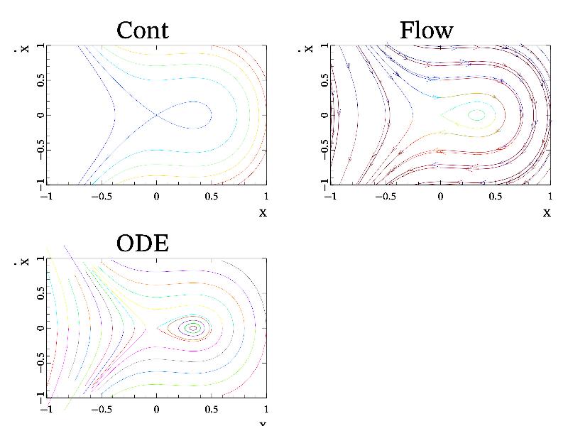
The simplest way to draw phase plain in MathGL is using flow function(s), which automatically select several points and draw flow threads. If the ODE have an integral of motion (like Hamiltonian H(x,x')=const for dissipation-free case) then you can use cont function for plotting isolines (contours). In fact. isolines are the same as flow threads, but without arrows on it. Finally, you can directly solve ODE using ode function and plot its numerical solution.

Let demonstrate this for ODE equation x''-x+3*x^2=0. This is nonlinear oscillator with square nonlinearity. It has integral H=y^2+2*x^3-x^2=Const. Also it have 2 typical stationary points: saddle at {x=0, y=0} and center at {x=1/3, y=0}. Motion at vicinity of center is just simple oscillations, and is stable to small variation of parameters. In opposite, motion around saddle point is non-stable to small variation of parameters, and is very slow. So, calculation around saddle points are more difficult, but more important. Saddle points are responsible for solitons, stochasticity and so on.

So, let draw this phase plain by 3 different methods. First, draw isolines for H=y^2+2*x^3-x^2=Const – this is simplest for ODE without dissipation. Next, draw flow threads – this is straightforward way, but the automatic choice of starting points is not always optimal. Finally, use ode to check the above plots. At this we need to run ode in both direction of time (in future and in the past) to draw whole plain. Alternatively, one can put starting points far from (or at the bounding box as done in flow) the plot, but this is a more complicated. The sample code is:

int sample(mglGraph *gr)
{
  gr->SubPlot(2,2,0,"<_");  gr->Title("Cont");  gr->Box();
  gr->Axis();  gr->Label('x',"x");  gr->Label('y',"\\dot{x}");
  mglData f(100,100);   gr->Fill(f,"y^2+2*x^3-x^2-0.5");
  gr->Cont(f);
  gr->SubPlot(2,2,1,"<_");  gr->Title("Flow");  gr->Box();
  gr->Axis();  gr->Label('x',"x");  gr->Label('y',"\\dot{x}");
  mglData fx(100,100), fy(100,100);
  gr->Fill(fx,"x-3*x^2");  gr->Fill(fy,"y");
  gr->Flow(fy,fx,"v","value 7");
  gr->SubPlot(2,2,2,"<_");  gr->Title("ODE");   gr->Box();
  gr->Axis();  gr->Label('x',"x");  gr->Label('y',"\\dot{x}");
  for(double x=-1;x<1;x+=0.1)
  {
    mglData in(2), r;   in.a[0]=x;
    r = mglODE("y;x-3*x^2","xy",in);
    gr->Plot(r.SubData(0), r.SubData(1));
    r = mglODE("-y;-x+3*x^2","xy",in);
    gr->Plot(r.SubData(0), r.SubData(1));
  }
}