---

3.5.10 Data interpolation ¶

There are many functions to get interpolated values of a data array. Basically all of them can be divided by 3 categories:

1. functions which return single value at given point (see Интерполяция and mglGSpline() in Глобальные функции);
2. functions subdata and evaluate for indirect access to data elements;
3. functions refill, gspline and datagrid which fill regular (rectangular) data array by interpolated values.

The usage of first category is rather straightforward and don’t need any special comments.

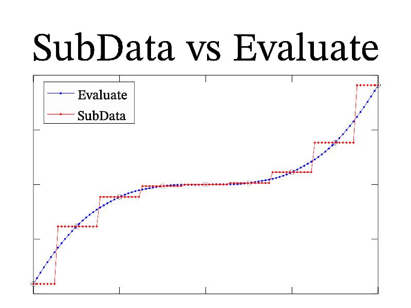
There is difference in indirect access functions. Function subdata use use step-like interpolation to handle correctly single nan values in the data array. Contrary, function evaluate use local spline interpolation, which give smoother output but spread nan values. So, subdata should be used for specific data elements (for example, for given column), and evaluate should be used for distributed elements (i.e. consider data array as some field). Following sample illustrates this difference:

int sample(mglGraph *gr)
{
  gr->SubPlot(1,1,0,"");  gr->Title("SubData vs Evaluate");
  mglData in(9), arg(99), e, s;
  gr->Fill(in,"x^3/1.1"); gr->Fill(arg,"4*x+4");
  gr->Plot(in,"ko ");     gr->Box();
  e = in.Evaluate(arg,false); gr->Plot(e,"b.","legend 'Evaluate'");
  s = in.SubData(arg);    gr->Plot(s,"r.","legend 'SubData'");
  gr->Legend(2);
}

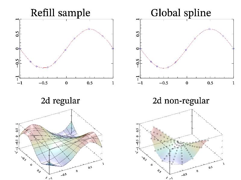
Example of datagrid usage is done in Making regular data. Here I want to show the peculiarities of refill and gspline functions. Both functions require argument(s) which provide coordinates of the data values, and return rectangular data array which equidistantly distributed in axis range. So, in opposite to evaluate function, refill and gspline can interpolate non-equidistantly distributed data. At this both functions refill and gspline provide continuity of 2nd derivatives along coordinate(s). However, refill is slower but give better (from human point of view) result than global spline gspline due to more advanced algorithm. Following sample illustrates this difference:

int sample(mglGraph *gr)
{
  mglData x(10), y(10), r(100);
  x.Modify("0.5+rnd");  x.CumSum("x");  x.Norm(-1,1);
  y.Modify("sin(pi*v)/1.5",x);
  gr->SubPlot(2,2,0,"<_");  gr->Title("Refill sample");
  gr->Axis();  gr->Box(); gr->Plot(x,y,"o ");
  gr->Refill(r,x,y);  // or you can use r.Refill(x,y,-1,1);
  gr->Plot(r,"r");  gr->FPlot("sin(pi*x)/1.5","B:");
  gr->SubPlot(2,2,1,"<_");gr->Title("Global spline");
  gr->Axis();  gr->Box(); gr->Plot(x,y,"o ");
  r.RefillGS(x,y,-1,1);   gr->Plot(r,"r");
  gr->FPlot("sin(pi*x)/1.5","B:");

  gr->Alpha(true);  gr->Light(true);
  mglData z(10,10), xx(10,10), yy(10,10), rr(100,100);
  y.Modify("0.5+rnd");  y.CumSum("x");  y.Norm(-1,1);
  for(int i=0;i<10;i++) for(int j=0;j<10;j++)
    z.a[i+10*j] = sin(M_PI*x.a[i]*y.a[j])/1.5;
  gr->SubPlot(2,2,2); gr->Title("2d regular");  gr->Rotate(40,60);
  gr->Axis();  gr->Box(); gr->Mesh(x,y,z,"k");
  gr->Refill(rr,x,y,z); gr->Surf(rr);

  gr->Fill(xx,"(x+1)/2*cos(y*pi/2-1)");
  gr->Fill(yy,"(x+1)/2*sin(y*pi/2-1)");
  for(int i=0;i<10*10;i++)
    z.a[i] = sin(M_PI*xx.a[i]*yy.a[i])/1.5;
  gr->SubPlot(2,2,3); gr->Title("2d non-regular");  gr->Rotate(40,60);
  gr->Axis();  gr->Box();  gr->Plot(xx,yy,z,"ko ");
  gr->Refill(rr,xx,yy,z);  gr->Surf(rr);
}