---

3.5.14 PDE solving hints ¶

Solving of Partial Differential Equations (PDE, including beam tracing) and ray tracing (or finding particle trajectory) are more or less common task. So, MathGL have several functions for that. There are ray for ray tracing, pde for PDE solving, qo2d for beam tracing in 2D case (see Глобальные функции). Note, that these functions take “Hamiltonian” or equations as string values. And I don’t plan now to allow one to use user-defined functions. There are 2 reasons: the complexity of corresponding interface; and the basic nature of used methods which are good for samples but may not good for serious scientific calculations.

The ray tracing can be done by ray function. Really ray tracing equation is Hamiltonian equation for 3D space. So, the function can be also used for finding a particle trajectory (i.e. solve Hamiltonian ODE) for 1D, 2D or 3D cases. The function have a set of arguments. First of all, it is Hamiltonian which defined the media (or the equation) you are planning to use. The Hamiltonian is defined by string which may depend on coordinates ‘x’, ‘y’, ‘z’, time ‘t’ (for particle dynamics) and momentums ‘p’=p_x, ‘q’=p_y, ‘v’=p_z. Next, you have to define the initial conditions for coordinates and momentums at ‘t’=0 and set the integrations step (default is 0.1) and its duration (default is 10). The Runge-Kutta method of 4-th order is used for integration.

  const char *ham = "p^2+q^2-x-1+i*0.5*(y+x)*(y>-x)";
  mglData r = mglRay(ham, mglPoint(-0.7, -1), mglPoint(0, 0.5), 0.02, 2);

This example calculate the reflection from linear layer (media with Hamiltonian ‘p^2+q^2-x-1’=p_x^2+p_y^2-x-1). This is parabolic curve. The resulting array have 7 columns which contain data for {x,y,z,p,q,v,t}.

The solution of PDE is a bit more complicated. As previous you have to specify the equation as pseudo-differential operator \hat H(x, \nabla) which is called sometime as “Hamiltonian” (for example, in beam tracing). As previously, it is defined by string which may depend on coordinates ‘x’, ‘y’, ‘z’ (but not time!), momentums ‘p’=(d/dx)/i k_0, ‘q’=(d/dy)/i k_0 and field amplitude ‘u’=|u|. The evolutionary coordinate is ‘z’ in all cases. So that, the equation look like du/dz = ik_0 H(x,y,\hat p, \hat q, |u|)[u]. Dependence on field amplitude ‘u’=|u| allows one to solve nonlinear problems too. For example, for nonlinear Shrodinger equation you may set ham="p^2 + q^2 - u^2". Also you may specify imaginary part for wave absorption, like ham = "p^2 + i*x*(x>0)" or ham = "p^2 + i1*x*(x>0)".

Next step is specifying the initial conditions at ‘z’ equal to minimal z-axis value. The function need 2 arrays for real and for imaginary part. Note, that coordinates x,y,z are supposed to be in specified axis range. So, the data arrays should have corresponding scales. Finally, you may set the integration step and parameter k0=k_0. Also keep in mind, that internally the 2 times large box is used (for suppressing numerical reflection from boundaries) and the equation should well defined even in this extended range.

Final comment is concerning the possible form of pseudo-differential operator H. At this moment, simplified form of operator H is supported – all “mixed” terms (like ‘x*p’->x*d/dx) are excluded. For example, in 2D case this operator is effectively H = f(p,z) + g(x,z,u). However commutable combinations (like ‘x*q’->x*d/dy) are allowed for 3D case.

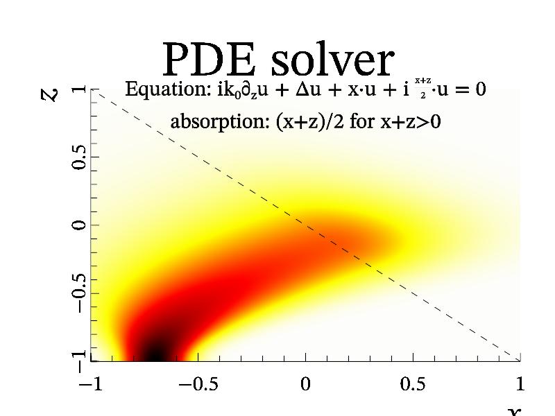
So, for example let solve the equation for beam deflected from linear layer and absorbed later. The operator will have the form ‘"p^2+q^2-x-1+i*0.5*(z+x)*(z>-x)"’ that correspond to equation 1/ik_0 * du/dz + d^2 u/dx^2 + d^2 u/dy^2 + x * u + i (x+z)/2 * u = 0. This is typical equation for Electron Cyclotron (EC) absorption in magnetized plasmas. For initial conditions let me select the beam with plane phase front exp(-48*(x+0.7)^2). The corresponding code looks like this:

int sample(mglGraph *gr)
{
  mglData a,re(128),im(128);
  gr->Fill(re,"exp(-48*(x+0.7)^2)");
  a = gr->PDE("p^2+q^2-x-1+i*0.5*(z+x)*(z>-x)", re, im, 0.01, 30);
  a.Transpose("yxz");
  gr->SubPlot(1,1,0,"<_"); gr->Title("PDE solver");
  gr->SetRange('c',0,1);  gr->Dens(a,"wyrRk");
  gr->Axis(); gr->Label('x', "\\i x");  gr->Label('y', "\\i z");
  gr->FPlot("-x", "k|");
  gr->Puts(mglPoint(0, 0.85), "absorption: (x+z)/2 for x+z>0");
  gr->Puts(mglPoint(0,1.1),"Equation: ik_0\\partial_zu + \\Delta u + x\\cdot u + i \\frac{x+z}{2}\\cdot u = 0");
  return 0;
}

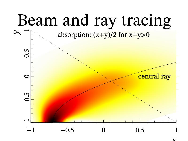
The next example is example of beam tracing. Beam tracing equation is special kind of PDE equation written in coordinates accompanied to a ray. Generally this is the same parameters and limitation as for PDE solving but the coordinates are defined by the ray and by parameter of grid width w in direction transverse the ray. So, you don’t need to specify the range of coordinates. BUT there is limitation. The accompanied coordinates are well defined only for smooth enough rays, i.e. then the ray curvature K (which is defined as 1/K^2 = (|r''|^2 |r'|^2 - (r'', r'')^2)/|r'|^6) is much large then the grid width: K>>w. So, you may receive incorrect results if this condition will be broken.

You may use following code for obtaining the same solution as in previous example:

int sample(mglGraph *gr)
{
  mglData r, xx, yy, a, im(128), re(128);
  const char *ham = "p^2+q^2-x-1+i*0.5*(y+x)*(y>-x)";
  r = mglRay(ham, mglPoint(-0.7, -1), mglPoint(0, 0.5), 0.02, 2);
  gr->SubPlot(1,1,0,"<_"); gr->Title("Beam and ray tracing");
  gr->Plot(r.SubData(0), r.SubData(1), "k");
  gr->Axis(); gr->Label('x', "\\i x");  gr->Label('y', "\\i z");

  // now start beam tracing
  gr->Fill(re,"exp(-48*x^2)");
  a = mglQO2d(ham, re, im, r, xx, yy, 1, 30);
  gr->SetRange('c',0, 1);
  gr->Dens(xx, yy, a, "wyrRk");
  gr->FPlot("-x", "k|");
  gr->Puts(mglPoint(0, 0.85), "absorption: (x+y)/2 for x+y>0");
  gr->Puts(mglPoint(0.7, -0.05), "central ray");
  return 0;
}

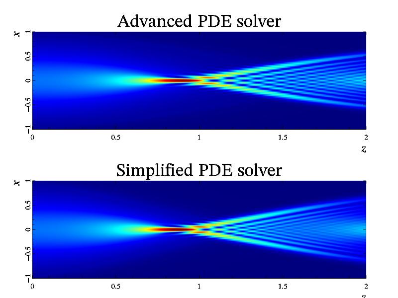
Note, the pde is fast enough and suitable for many cases routine. However, there is situations then media have both together: strong spatial dispersion and spatial inhomogeneity. In this, case the pde will produce incorrect result and you need to use advanced PDE solver apde. For example, a wave beam, propagated in plasma, described by Hamiltonian exp(-x^2-p^2), will have different solution for using of simplification and advanced PDE solver:

int sample(mglGraph *gr)
{
  gr->SetRanges(-1,1,0,2,0,2);
  mglData ar(256), ai(256);	gr->Fill(ar,"exp(-2*x^2)");

  mglData res1(gr->APDE("exp(-x^2-p^2)",ar,ai,0.01));	res1.Transpose();
  gr->SubPlot(1,2,0,"_");	gr->Title("Advanced PDE solver");
  gr->SetRanges(0,2,-1,1);	gr->SetRange('c',res1);
  gr->Dens(res1);	gr->Axis();	gr->Box();
  gr->Label('x',"\\i z");	gr->Label('y',"\\i x");
  gr->Puts(mglPoint(-0.5,0.2),"i\\partial_z\\i u = exp(-\\i x^2+\\partial_x^2)[\\i u]","y");

  mglData res2(gr->PDE("exp(-x^2-p^2)",ar,ai,0.01));
  gr->SubPlot(1,2,1,"_");	gr->Title("Simplified PDE solver");
  gr->Dens(res2);	gr->Axis();	gr->Box();
  gr->Label('x',"\\i z");	gr->Label('y',"\\i x");
  gr->Puts(mglPoint(-0.5,0.2),"i\\partial_z\\i u \\approx\\ exp(-\\i x^2)\\i u+exp(\\partial_x^2)[\\i u]","y");
  return 0;
}