This file documents the Mathematical Graphic Library (MathGL), a collection of classes and routines for scientific plotting. It corresponds to release 8.0 of the library. Please report any errors in this manual to mathgl.abalakin@gmail.org. More information about MathGL can be found at the project homepage, http://mathgl.sourceforge.net/.
Copyright © 2008-2012 Alexey A. Balakin.
Permission is granted to copy, distribute and/or modify this document under the terms of the GNU Free Documentation License, Version 1.2 or any later version published by the Free Software Foundation; with no Invariant Sections, no Front-Cover Texts, and no Back-Cover Texts. A copy of the license is included in the section entitled “GNU Free Documentation License.”
MathGL is ...
| • What is MathGL? | ||
| • MathGL features | ||
| • Installation | ||
| • Quick guide | ||
| • Changes from v.1 | ||
| • Utilities | ||
| • Thanks |
Next: MathGL features, Up: Overview [Contents][Index]
A code for making high-quality scientific graphics under Linux and Windows. A code for the fast handling and plotting of large data arrays. A code for working in window and console regimes and for easy including into another program. A code with large and renewal set of graphics. Exactly such a code I tried to put in MathGL library.
At this version (8.0) MathGL has more than 50 general types of graphics for 1d, 2d and 3d data arrays. It can export graphics to bitmap and vector (EPS or SVG) files. It has OpenGL interface and can be used from console programs. It has functions for data handling and script MGL language for simplification of data plotting. It also has several types of transparency and smoothed lighting, vector fonts and TeX-like symbol parsing, arbitrary curvilinear coordinate system and many other useful things (see pictures section at homepage). Finally it is platform-independent and free (under GPL v.2.0 or later license).
Next: Installation, Previous: What is MathGL?, Up: Overview [Contents][Index]
MathGL can plot a wide range of graphics. It includes:
In fact, I created the functions for drawing of all the types of scientific plots that I know. The list of plots is growing; if you need some special type of a plot then please email me e-mail and it will appear in the new version.
I tried to make plots as nice looking as possible: e.g., a surface can be transparent and highlighted by several (up to 10) light sources. Most of the drawing functions have 2 variants: simple one for the fast plotting of data, complex one for specifying of the exact position of the plot (including parametric representation). Resulting image can be saved in bitmap PNG, JPEG, GIF, TGA, BMP format, or in vector EPS, SVG or TeX format, or in 3D formats OBJ, OFF, STL, or in PRC format which can be converted into U3D.
All texts are drawn by vector fonts, which allows for high scalability and portability. Texts may contain commands for: some of the TeX-like symbols, changing index (upper or lower indexes) and the style of font inside the text string (see Font styles). Texts of ticks are rotated with axis rotation. It is possible to create a legend of plot and put text in an arbitrary position on the plot. Arbitrary text encoding (by the help of function setlocale()) and UTF-16 encoding are supported.
Special class mglData is used for data encapsulation (see Data processing). In addition to a safe creation and deletion of data arrays it includes functions for data processing (smoothing, differentiating, integrating, interpolating and so on) and reading of data files with automatic size determination. Class mglData can handle arrays with up to three dimensions (arrays which depend on up to 3 independent indexes a_{ijk}). Using an array with higher number of dimensions is not meaningful, because I do not know how it can be plotted. Data filling and modification may be done manually or by textual formulas.
There is fast evaluation of a textual mathematical expression (see Textual formulas). It is based on string precompilation to tree-like code at the creation of class instance. At evaluation stage code performs only fast tree-walk and returns the value of the expression. In addition to changing data values, textual formulas are also used for drawing in arbitrary curvilinear coordinates. A set of such curvilinear coordinates is limited only by user’s imagination rather than a fixed list like: polar, parabolic, spherical, and so on.
Next: Quick guide, Previous: MathGL features, Up: Overview [Contents][Index]
MathGL can be installed in 4 different ways.
cmake . twice, after it make and make install with root/sudo rights. Sometimes after installation you may need to update the library list – just execute ldconfig with root/sudo rights.
There are several additional options which are switched off by default. They are: enable-fltk, enable-glut, enable-qt4, enable-qt5 for ebabling FLTK, GLUT and/or Qt windows; enable-jpeg, enable-gif, enable-hdf5 and so on for enabling corresponding file formats; enable-all for enabling all additional features. For using double as base internal data type use option enable-double. For enabling language interfaces use enable-python, enable-octave or enable-all-swig for all languages. You can use WYSIWYG tool (cmake-gui) to view all of them, or type cmake -D enable-all=on -D enable-all-widgets=on -D enable-all-swig=on . in command line for enabling all features.
There is known bug for building in MinGW – you need to manually add linker option -fopenmp (i.e. CMAKE_EXE_LINKER_FLAGS:STRING='-fopenmp' and CMAKE_SHARED_LINKER_FLAGS:STRING='-fopenmp') if you enable OpenMP support (i.e. if enable-openmp=ON).
Note, you can download the latest sources (which can be not stable) from sourceforge.net SVN by command
svn checkout http://svn.code.sf.net/p/mathgl/code/mathgl-2x mathgl-code
IMPORTANT! MathGL use a set of defines, which were determined at configure stage and may differ if used with non-default compiler (like using MathGL binaries compiled by MinGW in VisualStudio). There are MGL_SYS_NAN, MGL_HAVE_TYPEOF, MGL_HAVE_PTHREAD, MGL_HAVE_ATTRIBUTE, MGL_HAVE_C99_COMPLEX, MGL_HAVE_RVAL. I specially set them to 0 for Borland and Microsoft compilers due to compatibility reasons. Also default setting are good for GNU (gcc, mingw) and clang compilers. However, for another compiler you may need to manually set this defines to 0 in file include/mgl2/config.h if you are using precompiled binaries.
Next: Changes from v.1, Previous: Installation, Up: Overview [Contents][Index]
There are 3 steps to prepare the plot in MathGL: (1) prepare data to be plotted, (2) setup plot, (3) plot data. Let me show this on the example of surface plotting.
First we need the data. MathGL use its own class mglData to handle data arrays (see Data processing). This class give ability to handle data arrays by more or less format independent way. So, create it
    int main()
    {
        mglData dat(30,40);	// data to for plotting
        for(long i=0;i<30;i++)   for(long j=0;j<40;j++)
            dat.a[i+30*j] = 1/(1+(i-15)*(i-15)/225.+(j-20)*(j-20)/400.);
Here I create matrix 30*40 and initialize it by formula. Note, that I use long type for indexes i, j because data arrays can be really large and long type will automatically provide proper indexing.
Next step is setup of the plot. The only setup I need is axis rotation and lighting.
        mglGraph gr;		// class for plot drawing
        gr.Rotate(50,60);	// rotate axis
        gr.Light(true);		// enable lighting
Everything is ready. And surface can be plotted.
gr.Surf(dat); // plot surface
Basically plot is done. But I decide to add yellow (‘y’ color, see Color styles) contour lines on the surface. To do it I can just add:
gr.Cont(dat,"y"); // plot yellow contour lines
This demonstrate one of base MathGL concept (see, General concepts) – “new drawing never clears things drawn already”. So, you can just consequently call different plotting functions to obtain “combined” plot. For example, if one need to draw axis then he can just call one more plotting function
gr.Axis(); // draw axis
Now picture is ready and we can save it in a file.
        gr.WriteFrame("sample.png");	// save it
    }
To compile your program, you need to specify the linker option -lmgl.
This is enough for a compilation of console program or with external (non-MathGL) window library. If you want to use FLTK or Qt windows provided by MathGL then you need to add the option -lmgl-wnd.
Fortran users also should add C++ library by the option -lstdc++. If library was built with enable-double=ON (this default for v.2.1 and later) then all real numbers must be real*8. You can make it automatic if use option -fdefault-real-8.
Next: Utilities, Previous: Quick guide, Up: Overview [Contents][Index]
There are a lot of changes for v.2. Here I denote only main of them.
mglconv, mglview).
Next: Thanks, Previous: Changes from v.1, Up: Overview [Contents][Index]
MathGL library provides several tools for parsing MGL scripts. There is tools saving it to bitmap or vectorial images (mglconv). Tool mglview show MGL script and allow to rotate and setup the image. Another feature of mglview is loading *.mgld files (see ExportMGLD()) for quick viewing 3d pictures.
Both tools have similar set of arguments. They can be name of script file or options. You can use ‘-’ as script name for using standard input (i.e. pipes). Options are:
Additionally mglconv have following options:
Also you can create animated GIF file or a set of JPEG files with names ‘frameNNNN.jpg’ (here ‘NNNN’ is frame index). Values of the parameter $0 for making animation can be specified inside the script by comment ##a val for each value val (one comment for one value) or by option(s) ‘-A val’. Also you can specify a cycle for animation by comment ##c v1 v2 dv or by option -C v1:v2:dv. In the case of found/specified animation parameters, tool will execute script several times – once for each value of $0.
MathGL also provide another simple tool mgl.cgi which parse MGL script from CGI request and send back produced PNG file. Usually this program should be placed in /usr/lib/cgi-bin/. But you need to put this program by yourself due to possible security issues and difference of Apache server settings.
Javascript interface was developed with support of DATADVANCE company.
Next: General concepts, Previous: Overview, Up: Top [Contents][Index]
This chapter contain information about basic and advanced MathGL, hints and samples for all types of graphics. I recommend you read first 2 sections one after another and at least look on Hints section. Also I recommend you to look at General concepts and FAQ.
Note, that MathGL v.2.* have only 2 end-user interfaces: one for C/Fortran and similar languages which don’t support classes, another one for C++/Python/Octave and similar languages which support classes. So, most of samples placed in this chapter can be run as is (after minor changes due to different syntaxes for different languages). For example, the C++ code
#include <mgl2/mgl.h>
int main()
{
  mglGraph gr;
  gr.FPlot("sin(pi*x)");
  gr.WriteFrame("test.png");
}
in Python will be as
from mathgl import *
gr = mglGraph();
gr.FPlot("sin(pi*x)");
gr.WriteFrame("test.png");
in Octave will be as (you need first execute mathgl; in newer Octave versions)
gr = mglGraph();
gr.FPlot("sin(pi*x)");
gr.WriteFrame("test.png");
in C will be as
#include <mgl2/mgl_cf.h>
int main()
{
  HMGL gr = mgl_create_graph(600,400);
  mgl_fplot(gr,"sin(pi*x)","","");
  mgl_write_frame(gr,"test.png","");
  mgl_delete_graph(gr);
}
in Fortran will be as
integer gr, mgl_create_graph
gr = mgl_create_graph(600,400);
call mgl_fplot(gr,'sin(pi*x)','','');
call mgl_write_frame(gr,'test.png','');
call mgl_delete_graph(gr);
and so on.
| • Basic usage | ||
| • Advanced usage | ||
| • Data handling | ||
| • Data plotting | ||
| • Hints | ||
| • FAQ |
Next: Advanced usage, Up: Examples [Contents][Index]
MathGL library can be used by several manners. Each has positive and negative sides:
Positive side is the possibility to view the plot at once and to modify it (rotate, zoom or switch on transparency or lighting) by hand or by mouse. Negative sides are: the need of X-terminal and limitation consisting in working with the only one set of data at a time.
Positive aspects are: batch processing of similar data set (for example, a set of resulting data files for different calculation parameters), running from the console program (including the cluster calculation), fast and automated drawing, saving pictures for further analysis (or demonstration). Negative sides are: the usage of the external program for picture viewing. Also, the data plotting is non-visual. So, you have to imagine the picture (view angles, lighting and so on) before the plotting. I recommend to use graphical window for determining the optimal parameters of plotting on the base of some typical data set. And later use these parameters for batch processing in console program.
In this case the programmer has more freedom in selecting the window libraries (not only FLTK, Qt or GLUT), in positioning and surroundings control and so on. I recommend to use such way for “stand alone” programs.
Here one can use a set of standard widgets which support export to many file formats, copying to clipboard, handle mouse and so on.
MathGL drawing can be created not only by object oriented languages (like, C++ or Python), but also by pure C or Fortran-like languages. The usage of last one is mostly identical to usage of classes (except the different function names). But there are some differences. C functions must have argument HMGL (for graphics) and/or HMDT (for data arrays) which specifies the object for drawing or manipulating (changing). Fortran users may regard these variables as integer. So, firstly the user has to create this object by function mgl_create_*() and has to delete it after the using by function mgl_delete_*().
Let me consider the aforesaid in more detail.
| • Using MathGL window | ||
| • Drawing to file | ||
| • Animation | ||
| • Drawing in memory | ||
| • Draw and calculate | ||
| • Using QMathGL | ||
| • OpenGL output | ||
| • MathGL and PyQt | ||
| • MathGL and MPI |
Next: Drawing to file, Up: Basic usage [Contents][Index]
The “interactive” way of drawing in MathGL consists in window creation with help of class mglQT, mglFLTK or mglGLUT (see Widget classes) and the following drawing in this window. There is a corresponding code:
#include <mgl2/qt.h>
int sample(mglGraph *gr)
{
  gr->Rotate(60,40);
  gr->Box();
  return 0;
}
//-----------------------------------------------------
int main(int argc,char **argv)
{
  mglQT gr(sample,"MathGL examples");
  return gr.Run();
}
Here callback function sample is defined. This function does all drawing. Other function main is entry point function for console program. For compilation, just execute the command
gcc test.cpp -lmgl-qt5 -lmgl
You can use "-lmgl-qt4" instead of "-lmgl-qt5", if Qt4 is installed.
Alternatively you can create yours own class inherited from mglDraw class and re-implement the function Draw() in it:
#include <mgl2/qt.h>
class Foo : public mglDraw
{
public:
  int Draw(mglGraph *gr);
};
//-----------------------------------------------------
int Foo::Draw(mglGraph *gr)
{
  gr->Rotate(60,40);
  gr->Box();
  return 0;
}
//-----------------------------------------------------
int main(int argc,char **argv)
{
  Foo foo;
  mglQT gr(&foo,"MathGL examples");
  return gr.Run();
}
Or use pure C-functions:
#include <mgl2/mgl_cf.h>
int sample(HMGL gr, void *)
{
  mgl_rotate(gr,60,40,0);
  mgl_box(gr);
}
int main(int argc,char **argv)
{
  HMGL gr;
  gr = mgl_create_graph_qt(sample,"MathGL examples",0,0);
  return mgl_qt_run();
/* generally I should call mgl_delete_graph() here,
 * but I omit it in main() function. */
}
The similar code can be written for mglGLUT window (function sample() is the same):
#include <mgl2/glut.h>
int main(int argc,char **argv)
{
  mglGLUT gr(sample,"MathGL examples");
  return 0;
}
The rotation, shift, zooming, switching on/off transparency and lighting can be done with help of tool-buttons (for mglQT, mglFLTK) or by hot-keys: ‘a’, ‘d’, ‘w’, ‘s’ for plot rotation, ‘r’ and ‘f’ switching on/off transparency and lighting. Press ‘x’ for exit (or closing the window).
In this example function sample rotates axes (Rotate(), see Subplots and rotation) and draws the bounding box (Box()). Drawing is placed in separate function since it will be used on demand when window canvas needs to be redrawn.
Next: Animation, Previous: Using MathGL window, Up: Basic usage [Contents][Index]
Another way of using MathGL library is the direct writing of the picture to the file. It is most usable for plot creation during long calculation or for using of small programs (like Matlab or Scilab scripts) for visualizing repetitive sets of data. But the speed of drawing is much higher in comparison with a script language.
The following code produces a bitmap PNG picture:
#include <mgl2/mgl.h>
int main(int ,char **)
{
  mglGraph gr;
  gr.Alpha(true);   gr.Light(true);
  sample(&gr);              // The same drawing function.
  gr.WritePNG("test.png");  // Don't forget to save the result!
  return 0;
}
For compilation, you need only libmgl library not the one with widgets
gcc test.cpp -lmgl
This can be important if you create a console program in computer/cluster where X-server (and widgets) is inaccessible.
The only difference from the previous variant (using windows) is manual switching on the transparency Alpha and lightning Light, if you need it. The usage of frames (see Animation) is not advisable since the whole image is prepared each time. If function sample contains frames then only last one will be saved to the file. In principle, one does not need to separate drawing functions in case of direct file writing in consequence of the single calling of this function for each picture. However, one may use the same drawing procedure to create a plot with changeable parameters, to export in different file types, to emphasize the drawing code and so on. So, in future I will put the drawing in the separate function.
The code for export into other formats (for example, into vector EPS file) looks the same:
#include <mgl2/mgl.h>
int main(int ,char **)
{
  mglGraph gr;
  gr.Light(true);
  sample(&gr);              // The same drawing function.
  gr.WriteEPS("test.eps");  // Don't forget to save the result!
  return 0;
}
The difference from the previous one is using other function WriteEPS() for EPS format instead of function WritePNG(). Also, there is no switching on of the plot transparency Alpha since EPS format does not support it.
Next: Drawing in memory, Previous: Drawing to file, Up: Basic usage [Contents][Index]
Widget classes (mglWindow, mglGLUT) support a delayed drawing, when all plotting functions are called once at the beginning of writing to memory lists. Further program displays the saved lists faster. Resulting redrawing will be faster but it requires sufficient memory. Several lists (frames) can be displayed one after another (by pressing ‘,’, ‘.’) or run as cinema. To switch these feature on one needs to modify function sample:
int sample(mglGraph *gr)
{
  gr->NewFrame();             // the first frame
  gr->Rotate(60,40);
  gr->Box();
  gr->EndFrame();             // end of the first frame
  gr->NewFrame();             // the second frame
  gr->Box();
  gr->Axis("xy");
  gr->EndFrame();             // end of the second frame
  return gr->GetNumFrame();   // returns the frame number
}
First, the function creates a frame by calling NewFrame() for rotated axes and draws the bounding box. The function EndFrame() must be called after the frame drawing! The second frame contains the bounding box and axes Axis("xy") in the initial (unrotated) coordinates. Function sample returns the number of created frames GetNumFrame().
Note, that animation can be also done as visualization of running calculations (see Draw and calculate).
Pictures with animation can be saved in file(s) as well. You can: export in animated GIF, or save each frame in separate file (usually JPEG) and convert these files into the movie (for example, by help of ImageMagic). Let me show both methods.
The simplest methods is making animated GIF. There are 3 steps: (1) open GIF file by StartGIF() function; (2) create the frames by calling NewFrame() before and EndFrame() after plotting; (3) close GIF by CloseGIF() function. So the simplest code for “running” sinusoid will look like this:
#include <mgl2/mgl.h>
int main(int ,char **)
{
  mglGraph gr;
  mglData dat(100);
  char str[32];
  gr.StartGIF("sample.gif");
  for(int i=0;i<40;i++)
  {
    gr.NewFrame();     // start frame
    gr.Box();          // some plotting
    for(int j=0;j<dat.nx;j++)
      dat.a[j]=sin(M_PI*j/dat.nx+M_PI*0.05*i);
    gr.Plot(dat,"b");
    gr.EndFrame();     // end frame
  }
  gr.CloseGIF();
  return 0;
}
The second way is saving each frame in separate file (usually JPEG) and later make the movie from them. MathGL have special function for saving frames – it is WriteFrame(). This function save each frame with automatic name ‘frame0001.jpg, frame0002.jpg’ and so on. Here prefix ‘frame’ is defined by PlotId variable of mglGraph class. So the similar code will look like this:
#include <mgl2/mgl.h>
int main(int ,char **)
{
  mglGraph gr;
  mglData dat(100);
  char str[32];
  for(int i=0;i<40;i++)
  {
    gr.NewFrame();     // start frame
    gr.Box();          // some plotting
    for(int j=0;j<dat.nx;j++)
      dat.a[j]=sin(M_PI*j/dat.nx+M_PI*0.05*i);
    gr.Plot(dat,"b");
    gr.EndFrame();     // end frame
    gr.WriteFrame();   // save frame
  }
  return 0;
}
Created files can be converted to movie by help of a lot of programs. For example, you can use ImageMagic (command ‘convert frame*.jpg movie.mpg’), MPEG library, GIMP and so on.
Finally, you can use mglconv tool for doing the same with MGL scripts (see Utilities).
Next: Draw and calculate, Previous: Animation, Up: Basic usage [Contents][Index]
The last way of MathGL using is the drawing in memory. Class mglGraph allows one to create a bitmap picture in memory. Further this picture can be displayed in window by some window libraries (like wxWidgets, FLTK, Windows GDI and so on). For example, the code for drawing in wxWidget library looks like:
void MyForm::OnPaint(wxPaintEvent& event)
{
  int w,h,x,y;
  GetClientSize(&w,&h);   // size of the picture
  mglGraph gr(w,h);

  gr.Alpha(true);         // draws something using MathGL
  gr.Light(true);
  sample(&gr,NULL);

  wxImage img(w,h,gr.GetRGB(),true);
  ToolBar->GetSize(&x,&y);    // gets a height of the toolbar if any
  wxPaintDC dc(this);         // and draws it
  dc.DrawBitmap(wxBitmap(img),0,y);
}
The drawing in other libraries is most the same.
For example, FLTK code will look like
void Fl_MyWidget::draw()
{
  mglGraph gr(w(),h());
  gr.Alpha(true);         // draws something using MathGL
  gr.Light(true);
  sample(&gr,NULL);
  fl_draw_image(gr.GetRGB(), x(), y(), gr.GetWidth(), gr.GetHeight(), 3);
}
Qt code will look like
void MyWidget::paintEvent(QPaintEvent *)
{
  mglGraph gr(w(),h());

  gr.Alpha(true);         // draws something using MathGL
  gr.Light(true);         gr.Light(0,mglPoint(1,0,-1));
  sample(&gr,NULL);

  // Qt don't support RGB format as is. So, let convert it to BGRN.
  long w=gr.GetWidth(), h=gr.GetHeight();
  unsigned char *buf = new uchar[4*w*h];
  gr.GetBGRN(buf, 4*w*h)
  QPixmap pic = QPixmap::fromImage(QImage(*buf, w, h, QImage::Format_RGB32));

  QPainter paint;
  paint.begin(this);  paint.drawPixmap(0,0,pic);  paint.end();
  delete []buf;
}
Next: Using QMathGL, Previous: Drawing in memory, Up: Basic usage [Contents][Index]
MathGL can be used to draw plots in parallel with some external calculations. The simplest way for this is the usage of mglDraw class. At this you should enable pthread for widgets by setting enable-pthr-widget=ON at configure stage (it is set by default).
First, you need to inherit you class from mglDraw class, define virtual members Draw() and Calc() which will draw the plot and proceed calculations. You may want to add the pointer mglWnd *wnd; to window with plot for interacting with them. Finally, you may add any other data or member functions. The sample class is shown below
class myDraw : public mglDraw
{
	mglPoint pnt;	// some variable for changeable data
	long i;			// another variable to be shown
	mglWnd *wnd;	// external window for plotting
public:
	myDraw(mglWnd *w=0) : mglDraw()	{	wnd=w;	}
	void SetWnd(mglWnd *w)	{	wnd=w;	}
	int Draw(mglGraph *gr)
	{
		gr->Line(mglPoint(),pnt,"Ar2");
		char str[16];	snprintf(str,15,"i=%ld",i);
		gr->Puts(mglPoint(),str);
		return 0;
	}
	void Calc()
	{
		for(i=0;;i++)	// do calculation
		{
			long_calculations();// which can be very long
			Check();	// check if need pause
			pnt.Set(2*mgl_rnd()-1,2*mgl_rnd()-1);
			if(wnd)	wnd->Update();
		}
	}
} dr;
There is only one issue here. Sometimes you may want to pause calculations to view result carefully, or save state, or change something. So, you need to provide a mechanism for pausing. Class mglDraw provide function Check(); which check if toolbutton with pause is pressed and wait until it will be released. This function should be called in a "safety" places, where you can pause the calculation (for example, at the end of time step). Also you may add call exit(0); at the end of Calc(); function for closing window and exit after finishing calculations.
Finally, you need to create a window itself and run calculations.
int main(int argc,char **argv)
{
	mglFLTK gr(&dr,"Multi-threading test");	// create window
	dr.SetWnd(&gr);	// pass window pointer to yours class
	dr.Run();	// run calculations
	gr.Run();	// run event loop for window
	return 0;
}
Note, that you can reach the similar functionality without using mglDraw class (i.e. even for pure C code).
mglFLTK *gr=NULL;	// pointer to window
void *calc(void *)	// function with calculations
{
	mglPoint pnt;	// some data for plot
	for(long i=0;;i++)		// do calculation
	{
		long_calculations();	// which can be very long
		pnt.Set(2*mgl_rnd()-1,2*mgl_rnd()-1);
		if(gr)
		{
			gr->Clf();			// make new drawing
			// draw something
			gr->Line(mglPoint(),pnt,"Ar2");
			char str[16];	snprintf(str,15,"i=%ld",i);
			gr->Puts(mglPoint(),str);
			// don't forgot to update window
			gr->Update();
		}
	}
}
int main(int argc,char **argv)
{
	static pthread_t thr;
	pthread_create(&thr,0,calc,0);	// create separate thread for calculations
	pthread_detach(thr);			// and detach it
	gr = new mglFLTK;	// now create window
	gr->Run();			// and run event loop
	return 0;
}
This sample is exactly the same as one with mglDraw class, but it don’t have functionality for pausing calculations. If you need it then you have to create global mutex (like pthread_mutex_t *mutex = pthread_mutex_init(&mutex,NULL);), set it to window (like gr->SetMutex(mutex);) and periodically check it at calculations (like pthread_mutex_lock(&mutex); pthread_mutex_unlock(&mutex);).
Finally, you can put the event-handling loop in separate instead of yours code by using RunThr() function instead of Run() one. Unfortunately, such method work well only for FLTK windows and only if pthread support was enabled. Such limitation come from the Qt requirement to be run in the primary thread only. The sample code will be:
int main(int argc,char **argv)
{
	mglFLTK gr("test");
	gr.RunThr();	// <-- need MathGL version which use pthread for widgets
	mglPoint pnt;	// some data
	for(int i=0;i<10;i++)	// do calculation
	{
		long_calculations();// which can be very long
		pnt.Set(2*mgl_rnd()-1,2*mgl_rnd()-1);
		gr.Clf();			// make new drawing
		gr.Line(mglPoint(),pnt,"Ar2");
		char str[10] = "i=0";	str[3] = '0'+i;
		gr->Puts(mglPoint(),str);
		gr.Update();		// update window
	}
	return 0;	// finish calculations and close the window
}
Next: OpenGL output, Previous: Draw and calculate, Up: Basic usage [Contents][Index]
MathGL have several interface widgets for different widget libraries. There are QMathGL for Qt, Fl_MathGL for FLTK. These classes provide control which display MathGL graphics. Unfortunately there is no uniform interface for widget classes because all libraries have slightly different set of functions, features and so on. However the usage of MathGL widgets is rather simple. Let me show it on the example of QMathGL.
First of all you have to define the drawing function or inherit a class from mglDraw class. After it just create a window and setup QMathGL instance as any other Qt widget:
#include <QApplication>
#include <QMainWindow>
#include <QScrollArea>
#include <mgl2/qmathgl.h>
int main(int argc,char **argv)
{
  QApplication a(argc,argv);
  QMainWindow *Wnd = new QMainWindow;
  Wnd->resize(810,610);  // for fill up the QMGL, menu and toolbars
  Wnd->setWindowTitle("QMathGL sample");
  // here I allow to scroll QMathGL -- the case
  // then user want to prepare huge picture
  QScrollArea *scroll = new QScrollArea(Wnd);

  // Create and setup QMathGL
  QMathGL *QMGL = new QMathGL(Wnd);
//QMGL->setPopup(popup); // if you want to setup popup menu for QMGL
  QMGL->setDraw(sample);
  // or use QMGL->setDraw(foo); for instance of class Foo:public mglDraw
  QMGL->update();

  // continue other setup (menu, toolbar and so on)
  scroll->setWidget(QMGL);
  Wnd->setCentralWidget(scroll);
  Wnd->show();
  return a.exec();
}
Next: MathGL and PyQt, Previous: Using QMathGL, Up: Basic usage [Contents][Index]
MathGL have possibility to draw resulting plot using OpenGL. This produce resulting plot a bit faster, but with some limitations (especially at use of transparency and lighting). Generally, you need to prepare OpenGL window and call MathGL functions to draw it. There is GLUT interface (see Widget classes) to do it by simple way. Below I show example of OpenGL usage basing on Qt libraries (i.e. by using QGLWidget widget).
First, one need to define widget class derived from QGLWidget and implement a few methods: resizeGL() called after each window resize, paintGL() for displaying the image on the screen, and initializeGL() for initializing OpenGL. The header file looks as following.
#ifndef MAINWINDOW_H
#define MAINWINDOW_H

#include <QGLWidget>
#include <mgl2/mgl.h>

class MainWindow : public QGLWidget
{
  Q_OBJECT
protected:
  mglGraph *gr;         // pointer to MathGL core class
  void resizeGL(int nWidth, int nHeight);   // Method called after each window resize
  void paintGL();       // Method to display the image on the screen
  void initializeGL();  // Method to initialize OpenGL
public:
  MainWindow(QWidget *parent = 0);
  ~MainWindow();
};
#endif // MAINWINDOW_H
The class implementation is rather straightforward. One need to recreate the instance of mglGraph at initializing OpenGL, and ask MathGL to use OpenGL output (set argument 1 in mglGraph constructor). Of course, the mglGraph object should be deleted at destruction. The method resizeGL() just pass new sizes to OpenGL and update viewport sizes. All plotting functions are located in the method paintGL(). At this, one need to add 2 calls: gr->Clf() at beginning for clearing previous OpenGL primitives; and swapBuffers() for showing output on the screen. The source file looks as following.
#include "qgl_example.h"
#include <QApplication>
//#include <QtOpenGL>
//-----------------------------------------------------------------------------
MainWindow::MainWindow(QWidget *parent) : QGLWidget(parent)	{	gr=0;	}
//-----------------------------------------------------------------------------
MainWindow::~MainWindow()	{	if(gr)	delete gr;	}
//-----------------------------------------------------------------------------
void MainWindow::initializeGL()	// recreate instance of MathGL core
{
	if(gr)	delete gr;
	gr = new mglGraph(1);	// use '1' for argument to force OpenGL output in MathGL
}
//-----------------------------------------------------------------------------
void MainWindow::resizeGL(int w, int h) // standard resize replace
{
	QGLWidget::resizeGL(w, h);
	glViewport (0, 0, w, h);
}
//-----------------------------------------------------------------------------
void MainWindow::paintGL()	// main drawing function
{
	gr->Clf();	// clear previous OpenGL primitives
	gr->SubPlot(1,1,0);
	gr->Rotate(40,60);
	gr->Light(true);
	gr->AddLight(0,mglPoint(0,0,10),mglPoint(0,0,-1));
	gr->Axis();
	gr->Box();
	gr->FPlot("sin(pi*x)","i2");
	gr->FPlot("cos(pi*x)","|");
	gr->FSurf("cos(2*pi*(x^2+y^2))");
	gr->Finish();
	swapBuffers();	// show output on the screen
}
//-----------------------------------------------------------------------------
int main(int argc, char *argv[])	// create application
{
	mgl_textdomain(argv?argv[0]:NULL,"");
	QApplication a(argc, argv);
	MainWindow w;
	w.show();
	return a.exec();
}
//-----------------------------------------------------------------------------
Next: MathGL and MPI, Previous: OpenGL output, Up: Basic usage [Contents][Index]
Generally SWIG based classes (including the Python one) are the same as C++ classes. However, there are few tips for using MathGL with PyQt. Below I place a very simple python code which demonstrate how MathGL can be used with PyQt. This code is mostly written by Prof. Dr. Heino Falcke. You can just copy it to a file mgl-pyqt-test.py and execute it from python shell by command execfile("mgl-pyqt-test.py")
from PyQt4 import QtGui,QtCore
from mathgl import *
import sys
app = QtGui.QApplication(sys.argv)
qpointf=QtCore.QPointF()

class hfQtPlot(QtGui.QWidget):
    def __init__(self, parent=None):
        QtGui.QWidget.__init__(self, parent)
        self.img=(QtGui.QImage())
    def setgraph(self,gr):
        self.buffer='\t'
        self.buffer=self.buffer.expandtabs(4*gr.GetWidth()*gr.GetHeight())
        gr.GetBGRN(self.buffer,len(self.buffer))
        self.img=QtGui.QImage(self.buffer, gr.GetWidth(),gr.GetHeight(),QtGui.QImage.Format_ARGB32)
        self.update()
    def paintEvent(self, event):
        paint = QtGui.QPainter()
        paint.begin(self)
        paint.drawImage(qpointf,self.img)
        paint.end()

BackgroundColor=[1.0,1.0,1.0]
size=100
gr=mglGraph()
y=mglData(size)
#y.Modify("((0.7*cos(2*pi*(x+.2)*500)+0.3)*(rnd*0.5+0.5)+362.135+10000.)")
y.Modify("(cos(2*pi*x*10)+1.1)*1000.*rnd-501")
x=mglData(size)
x.Modify("x^2");

def plotpanel(gr,x,y,n):
    gr.SubPlot(2,2,n)
    gr.SetXRange(x)
    gr.SetYRange(y)
    gr.AdjustTicks()
    gr.Axis()
    gr.Box()
    gr.Label("x","x-Axis",1)
    gr.Label("y","y-Axis",1)
    gr.ClearLegend()
    gr.AddLegend("Legend: "+str(n),"k")
    gr.Legend()
    gr.Plot(x,y)


gr.Clf(BackgroundColor[0],BackgroundColor[1],BackgroundColor[2])
gr.SetPlotFactor(1.5)
plotpanel(gr,x,y,0)
y.Modify("(cos(2*pi*x*10)+1.1)*1000.*rnd-501")
plotpanel(gr,x,y,1)
y.Modify("(cos(2*pi*x*10)+1.1)*1000.*rnd-501")
plotpanel(gr,x,y,2)
y.Modify("(cos(2*pi*x*10)+1.1)*1000.*rnd-501")
plotpanel(gr,x,y,3)

gr.WritePNG("test.png","Test Plot")

qw = hfQtPlot()
qw.show()
qw.setgraph(gr)
qw.raise_()
Previous: MathGL and PyQt, Up: Basic usage [Contents][Index]
For using MathGL in MPI program you just need to: (1) plot its own part of data for each running node; (2) collect resulting graphical information in a single program (for example, at node with rank=0); (3) save it. The sample code below demonstrate this for very simple sample of surface drawing.
First you need to initialize MPI
#include <stdio.h>
#include <mgl2/mpi.h>
#include <mpi.h>

int main(int argc, char *argv[])
{
  // initialize MPI
  int rank=0, numproc=1;
  MPI_Init(&argc, &argv);
  MPI_Comm_size(MPI_COMM_WORLD,&numproc);
  MPI_Comm_rank(MPI_COMM_WORLD,&rank);
  if(rank==0) printf("Use %d processes.\n", numproc);
Next step is data creation. For simplicity, I create data arrays with the same sizes for all nodes. At this, you have to create mglGraph object too.
  // initialize data similarly for all nodes
  mglData a(128,256);
  mglGraphMPI gr;
Now, data should be filled by numbers. In real case, it should be some kind of calculations. But I just fill it by formula.
  // do the same plot for its own range
  char buf[64];
  sprintf(buf,"xrange %g %g",2.*rank/numproc-1,2.*(rank+1)/numproc-1);
  gr.Fill(a,"sin(2*pi*x)",buf);
It is time to plot the data. Don’t forget to set proper axis range(s) by using parametric form or by using options (as in the sample).
  // plot data in each node
  gr.Clf();   // clear image before making the image
  gr.Rotate(40,60);
  gr.Surf(a,"",buf);
Finally, let send graphical information to node with rank=0.
  // collect information
  if(rank!=0) gr.MPI_Send(0);
  else for(int i=1;i<numproc;i++)  gr.MPI_Recv(i);
Now, node with rank=0 have whole image. It is time to save the image to a file. Also, you can add a kind of annotations here – I draw axis and bounding box in the sample.
  if(rank==0)
  {
    gr.Box();   gr.Axis();   // some post processing
    gr.WritePNG("test.png"); // save result
  }
In my case the program is done, and I finalize MPI. In real program, you can repeat the loop of data calculation and data plotting as many times as you need.
  MPI_Finalize();
  return 0;
}
You can type ‘mpic++ test.cpp -lmgl-mpi -lmgl && mpirun -np 8 ./a.out’ for compilation and running the sample program on 8 nodes. Note, that you have to set enable-mpi=ON at MathGL configure to use this feature.
Next: Data handling, Previous: Basic usage, Up: Examples [Contents][Index]
Now I show several non-obvious features of MathGL: several subplots in a single picture, curvilinear coordinates, text printing and so on. Generally you may miss this section at first reading.
| • Subplots | ||
| • Axis and ticks | ||
| • Curvilinear coordinates | ||
| • Colorbars | ||
| • Bounding box | ||
| • Ternary axis | ||
| • Text features | ||
| • Legend sample | ||
| • Cutting sample |
Next: Axis and ticks, Up: Advanced usage [Contents][Index]
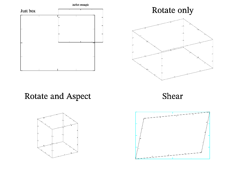
Let me demonstrate possibilities of plot positioning and rotation. MathGL has a set of functions: subplot, inplot, title, aspect and rotate and so on (see Subplots and rotation). The order of their calling is strictly determined. First, one changes the position of plot in image area (functions subplot, inplot and multiplot). Secondly, you can add the title of plot by title function. After that one may rotate the plot (function rotate). Finally, one may change aspects of axes (function aspect). The following code illustrates the aforesaid it:
int sample(mglGraph *gr)
{
  gr->SubPlot(2,2,0); gr->Box();
  gr->Puts(mglPoint(-1,1.1),"Just box",":L");
  gr->InPlot(0.2,0.5,0.7,1,false);  gr->Box();
  gr->Puts(mglPoint(0,1.2),"InPlot example");
  gr->SubPlot(2,2,1); gr->Title("Rotate only");
  gr->Rotate(50,60);  gr->Box();
  gr->SubPlot(2,2,2); gr->Title("Rotate and Aspect");
  gr->Rotate(50,60);  gr->Aspect(1,1,2);  gr->Box();
  gr->SubPlot(2,2,3); gr->Title("Shear");
  gr->Box("c"); gr->Shear(0.2,0.1); gr->Box();
  return 0;
}
Here I used function Puts for printing the text in arbitrary position of picture (see Text printing). Text coordinates and size are connected with axes. However, text coordinates may be everywhere, including the outside the bounding box. I’ll show its features later in Text features.
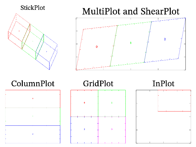
More complicated sample show how to use most of positioning functions:
int sample(mglGraph *gr)
{
  gr->SubPlot(3,2,0); gr->Title("StickPlot");
  gr->StickPlot(3, 0, 20, 30);  gr->Box("r"); gr->Puts(mglPoint(0),"0","r");
  gr->StickPlot(3, 1, 20, 30);  gr->Box("g"); gr->Puts(mglPoint(0),"1","g");
  gr->StickPlot(3, 2, 20, 30);  gr->Box("b"); gr->Puts(mglPoint(0),"2","b");
  gr->SubPlot(3,2,3,"");  gr->Title("ColumnPlot");
  gr->ColumnPlot(3, 0); gr->Box("r"); gr->Puts(mglPoint(0),"0","r");
  gr->ColumnPlot(3, 1); gr->Box("g"); gr->Puts(mglPoint(0),"1","g");
  gr->ColumnPlot(3, 2); gr->Box("b"); gr->Puts(mglPoint(0),"2","b");
  gr->SubPlot(3,2,4,"");  gr->Title("GridPlot");
  gr->GridPlot(2, 2, 0);  gr->Box("r"); gr->Puts(mglPoint(0),"0","r");
  gr->GridPlot(2, 2, 1);  gr->Box("g"); gr->Puts(mglPoint(0),"1","g");
  gr->GridPlot(2, 2, 2);  gr->Box("b"); gr->Puts(mglPoint(0),"2","b");
  gr->GridPlot(2, 2, 3);  gr->Box("m"); gr->Puts(mglPoint(0),"3","m");
  gr->SubPlot(3,2,5,"");  gr->Title("InPlot");  gr->Box();
  gr->InPlot(0.4, 1, 0.6, 1, true); gr->Box("r");
  gr->MultiPlot(3,2,1, 2, 1,"");  gr->Title("MultiPlot and ShearPlot"); gr->Box();
  gr->ShearPlot(3, 0, 0.2, 0.1);  gr->Box("r"); gr->Puts(mglPoint(0),"0","r");
  gr->ShearPlot(3, 1, 0.2, 0.1);  gr->Box("g"); gr->Puts(mglPoint(0),"1","g");
  gr->ShearPlot(3, 2, 0.2, 0.1);  gr->Box("b"); gr->Puts(mglPoint(0),"2","b");
  return 0;
}
Next: Curvilinear coordinates, Previous: Subplots, Up: Advanced usage [Contents][Index]
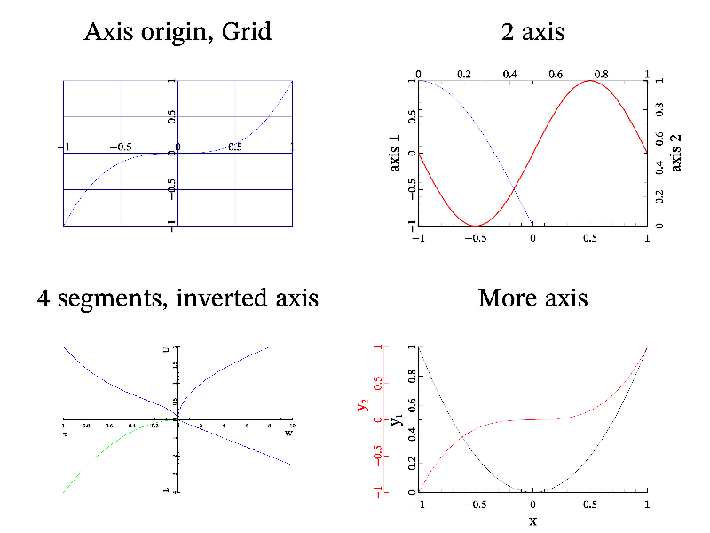
MathGL library can draw not only the bounding box but also the axes, grids, labels and so on. The ranges of axes and their origin (the point of intersection) are determined by functions SetRange(), SetRanges(), SetOrigin() (see Ranges (bounding box)). Ticks on axis are specified by function SetTicks, SetTicksVal, SetTicksTime (see Ticks). But usually
Function axis draws axes. Its textual string shows in which directions the axis or axes will be drawn (by default "xyz", function draws axes in all directions). Function grid draws grid perpendicularly to specified directions. Example of axes and grid drawing is:
int sample(mglGraph *gr)
{
  gr->SubPlot(2,2,0); gr->Title("Axis origin, Grid"); gr->SetOrigin(0,0);
  gr->Axis(); gr->Grid(); gr->FPlot("x^3");

  gr->SubPlot(2,2,1); gr->Title("2 axis");
  gr->SetRanges(-1,1,-1,1); gr->SetOrigin(-1,-1,-1);  // first axis
  gr->Axis(); gr->Label('y',"axis 1",0);  gr->FPlot("sin(pi*x)");
  gr->SetRanges(0,1,0,1);   gr->SetOrigin(1,1,1);   // second axis
  gr->Axis(); gr->Label('y',"axis 2",0);  gr->FPlot("cos(pi*x)");

  gr->SubPlot(2,2,3); gr->Title("More axis");
  gr->SetOrigin(NAN,NAN); gr->SetRange('x',-1,1);
  gr->Axis(); gr->Label('x',"x",0); gr->Label('y',"y_1",0);
  gr->FPlot("x^2","k");
  gr->SetRanges(-1,1,-1,1); gr->SetOrigin(-1.3,-1); // second axis
  gr->Axis("y","r");  gr->Label('y',"#r{y_2}",0.2);
  gr->FPlot("x^3","r");

  gr->SubPlot(2,2,2); gr->Title("4 segments, inverted axis");
  gr->SetOrigin(0,0);
  gr->InPlot(0.5,1,0.5,1);  gr->SetRanges(0,10,0,2);  gr->Axis();
  gr->FPlot("sqrt(x/2)");   gr->Label('x',"W",1); gr->Label('y',"U",1);
  gr->InPlot(0,0.5,0.5,1);  gr->SetRanges(1,0,0,2); gr->Axis("x");
  gr->FPlot("sqrt(x)+x^3"); gr->Label('x',"\\tau",-1);
  gr->InPlot(0.5,1,0,0.5);  gr->SetRanges(0,10,4,0);  gr->Axis("y");
  gr->FPlot("x/4"); gr->Label('y',"L",-1);
  gr->InPlot(0,0.5,0,0.5);  gr->SetRanges(1,0,4,0); gr->FPlot("4*x^2");
  return 0;
}
Note, that MathGL can draw not only single axis (which is default). But also several axis on the plot (see right plots). The idea is that the change of settings does not influence on the already drawn graphics. So, for 2-axes I setup the first axis and draw everything concerning it. Then I setup the second axis and draw things for the second axis. Generally, the similar idea allows one to draw rather complicated plot of 4 axis with different ranges (see bottom left plot).
At this inverted axis can be created by 2 methods. First one is used in this sample – just specify minimal axis value to be large than maximal one. This method work well for 2D axis, but can wrongly place labels in 3D case. Second method is more general and work in 3D case too – just use aspect function with negative arguments. For example, following code will produce exactly the same result for 2D case, but 2nd variant will look better in 3D.
// variant 1
gr->SetRanges(0,10,4,0);  gr->Axis();

// variant 2
gr->SetRanges(0,10,0,4);  gr->Aspect(1,-1);   gr->Axis();
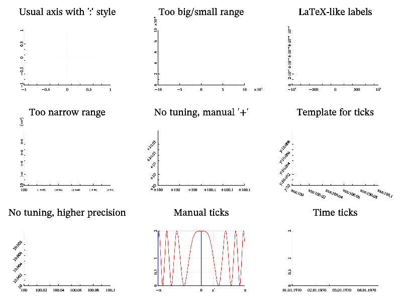
Another MathGL feature is fine ticks tunning. By default (if it is not changed by SetTicks function), MathGL try to adjust ticks positioning, so that they looks most human readable. At this, MathGL try to extract common factor for too large or too small axis ranges, as well as for too narrow ranges. Last one is non-common notation and can be disabled by SetTuneTicks function.
Also, one can specify its own ticks with arbitrary labels by help of SetTicksVal function. Or one can set ticks in time format. In last case MathGL will try to select optimal format for labels with automatic switching between years, months/days, hours/minutes/seconds or microseconds. However, you can specify its own time representation using formats described in http://www.manpagez.com/man/3/strftime/. Most common variants are ‘%X’ for national representation of time, ‘%x’ for national representation of date, ‘%Y’ for year with century.
The sample code, demonstrated ticks feature is
int sample(mglGraph *gr)
{
  gr->SubPlot(3,3,0); gr->Title("Usual axis");  gr->Axis();
  gr->SubPlot(3,3,1); gr->Title("Too big/small range");
  gr->SetRanges(-1000,1000,0,0.001);  gr->Axis();
  gr->SubPlot(3,3,2); gr->Title("LaTeX-like labels");
  gr->Axis("F!");
  gr->SubPlot(3,3,3); gr->Title("Too narrow range");
  gr->SetRanges(100,100.1,10,10.01);  gr->Axis();
  gr->SubPlot(3,3,4); gr->Title("No tuning, manual '+'");
  // for version<2.3 you need first call gr->SetTuneTicks(0);
  gr->Axis("+!");
  gr->SubPlot(3,3,5); gr->Title("Template for ticks");
  gr->SetTickTempl('x',"xxx:%g"); gr->SetTickTempl('y',"y:%g");
  gr->Axis();
  // now switch it off for other plots
  gr->SetTickTempl('x',"");   gr->SetTickTempl('y',"");
  gr->SubPlot(3,3,6); gr->Title("No tuning, higher precision");
  gr->Axis("!4");
  gr->SubPlot(3,3,7); gr->Title("Manual ticks");  gr->SetRanges(-M_PI,M_PI, 0, 2);
  gr->SetTicks('x',M_PI,0,0,"\\pi");  gr->AddTick('x',0.886,"x^*");
  // alternatively you can use following lines
  //double val[]={-M_PI, -M_PI/2, 0, 0.886, M_PI/2, M_PI};
  //gr->SetTicksVal('x', mglData(6,val), "-\\pi\n-\\pi/2\n0\nx^*\n\\pi/2\n\\pi");
  gr->Axis();  gr->Grid();  gr->FPlot("2*cos(x^2)^2", "r2");
  gr->SubPlot(3,3,8); gr->Title("Time ticks");  gr->SetRange('x',0,3e5);
  gr->SetTicksTime('x',0);  gr->Axis();
}
The last sample I want to show in this subsection is Log-axis. From MathGL’s point of view, the log-axis is particular case of general curvilinear coordinates. So, we need first define new coordinates (see also Curvilinear coordinates) by help of SetFunc or SetCoor functions. At this one should wary about proper axis range. So the code looks as following:
int sample(mglGraph *gr)
{
  gr->SubPlot(2,2,0,"<_");  gr->Title("Semi-log axis");
  gr->SetRanges(0.01,100,-1,1); gr->SetFunc("lg(x)","");
  gr->Axis(); gr->Grid("xy","g"); gr->FPlot("sin(1/x)");
  gr->Label('x',"x",0); gr->Label('y', "y = sin 1/x",0);

  gr->SubPlot(2,2,1,"<_");  gr->Title("Log-log axis");
  gr->SetRanges(0.01,100,0.1,100);  gr->SetFunc("lg(x)","lg(y)");
  gr->Axis(); gr->Grid("!","h=");   gr->Grid();
  gr->FPlot("sqrt(1+x^2)"); gr->Label('x',"x",0);
  gr->Label('y', "y = \\sqrt{1+x^2}",0);

  gr->SubPlot(2,2,2,"<_");  gr->Title("Minus-log axis");
  gr->SetRanges(-100,-0.01,-100,-0.1);  gr->SetFunc("-lg(-x)","-lg(-y)");
  gr->Axis(); gr->FPlot("-sqrt(1+x^2)");
  gr->Label('x',"x",0); gr->Label('y', "y = -\\sqrt{1+x^2}",0);

  gr->SubPlot(2,2,3,"<_");  gr->Title("Log-ticks");
  gr->SetRanges(0.1,100,0,100); gr->SetFunc("sqrt(x)","");
  gr->Axis(); gr->FPlot("x");
  gr->Label('x',"x",1); gr->Label('y', "y = x",0);
  return 0;
}
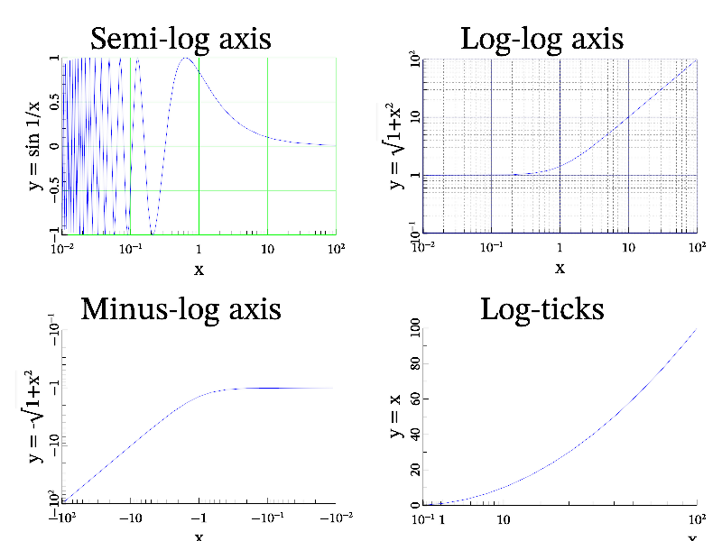
You can see that MathGL automatically switch to log-ticks as we define log-axis formula (in difference from v.1.*). Moreover, it switch to log-ticks for any formula if axis range will be large enough (see right bottom plot). Another interesting feature is that you not necessary define usual log-axis (i.e. when coordinates are positive), but you can define “minus-log” axis when coordinate is negative (see left bottom plot).
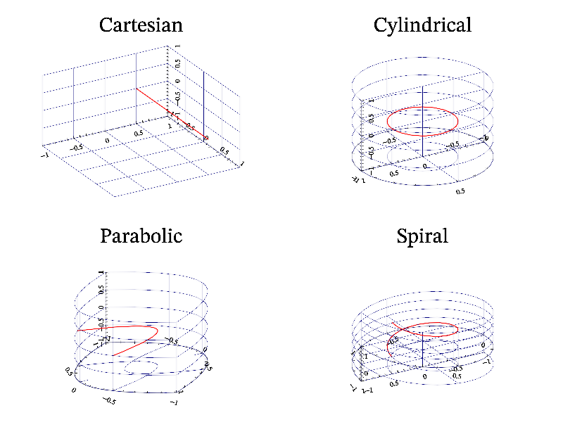
Next: Colorbars, Previous: Axis and ticks, Up: Advanced usage [Contents][Index]
As I noted in previous subsection, MathGL support curvilinear coordinates. In difference from other plotting programs and libraries, MathGL uses textual formulas for connection of the old (data) and new (output) coordinates. This allows one to plot in arbitrary coordinates. The following code plots the line y=0, z=0 in Cartesian, polar, parabolic and spiral coordinates:
int sample(mglGraph *gr)
{
  gr->SetOrigin(-1,1,-1);

  gr->SubPlot(2,2,0); gr->Title("Cartesian"); gr->Rotate(50,60);
  gr->FPlot("2*t-1","0.5","0","r2");
  gr->Axis(); gr->Grid();

  gr->SetFunc("y*sin(pi*x)","y*cos(pi*x)",0);
  gr->SubPlot(2,2,1); gr->Title("Cylindrical"); gr->Rotate(50,60);
  gr->FPlot("2*t-1","0.5","0","r2");
  gr->Axis(); gr->Grid();

  gr->SetFunc("2*y*x","y*y - x*x",0);
  gr->SubPlot(2,2,2); gr->Title("Parabolic"); gr->Rotate(50,60);
  gr->FPlot("2*t-1","0.5","0","r2");
  gr->Axis(); gr->Grid();

  gr->SetFunc("y*sin(pi*x)","y*cos(pi*x)","x+z");
  gr->SubPlot(2,2,3); gr->Title("Spiral");  gr->Rotate(50,60);
  gr->FPlot("2*t-1","0.5","0","r2");
  gr->Axis(); gr->Grid();
  gr->SetFunc(0,0,0); // set to default Cartesian
  return 0;
}
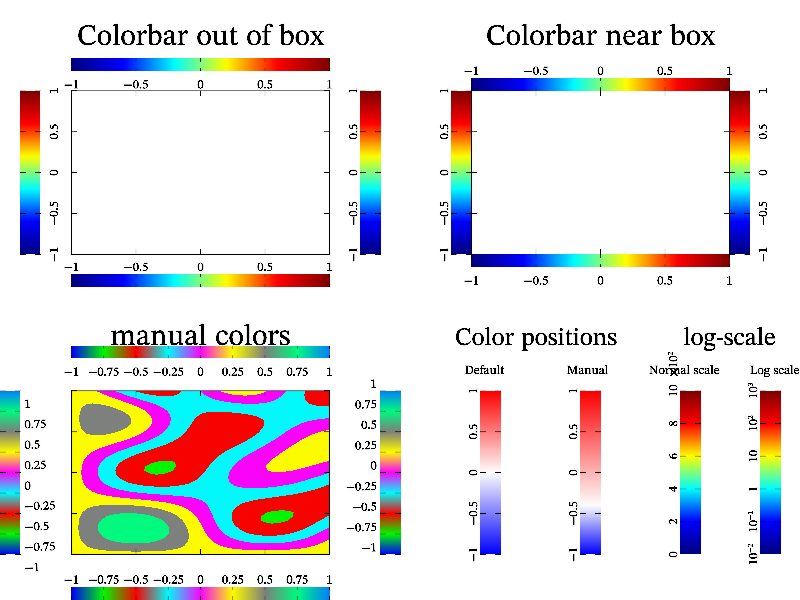
Next: Bounding box, Previous: Curvilinear coordinates, Up: Advanced usage [Contents][Index]
MathGL handle colorbar as special kind of axis. So, most of functions for axis and ticks setup will work for colorbar too. Colorbars can be in log-scale, and generally as arbitrary function scale; common factor of colorbar labels can be separated; and so on.
But of course, there are differences – colorbars usually located out of bounding box. At this, colorbars can be at subplot boundaries (by default), or at bounding box (if symbol ‘I’ is specified). Colorbars can handle sharp colors. And they can be located at arbitrary position too. The sample code, which demonstrate colorbar features is:
int sample(mglGraph *gr)
{
  gr->SubPlot(2,2,0); gr->Title("Colorbar out of box"); gr->Box();
  gr->Colorbar("<");  gr->Colorbar(">");
  gr->Colorbar("_");  gr->Colorbar("^");

  gr->SubPlot(2,2,1); gr->Title("Colorbar near box");   gr->Box();
  gr->Colorbar("<I"); gr->Colorbar(">I");
  gr->Colorbar("_I"); gr->Colorbar("^I");

  gr->SubPlot(2,2,2); gr->Title("manual colors");
  mglData a,v;  mgls_prepare2d(&a,0,&v);
  gr->Box();  gr->ContD(v,a);
  gr->Colorbar(v,"<");  gr->Colorbar(v,">");
  gr->Colorbar(v,"_");  gr->Colorbar(v,"^");

  gr->SubPlot(2,2,3);   gr->Title(" ");
  gr->Puts(mglPoint(-0.5,1.55),"Color positions",":C",-2);
  gr->Colorbar("bwr>",0.25,0);  gr->Puts(mglPoint(-0.9,1.2),"Default");
  gr->Colorbar("b{w,0.3}r>",0.5,0); gr->Puts(mglPoint(-0.1,1.2),"Manual");

  gr->Puts(mglPoint(1,1.55),"log-scale",":C",-2);
  gr->SetRange('c',0.01,1e3);
  gr->Colorbar(">",0.75,0);  gr->Puts(mglPoint(0.65,1.2),"Normal scale");
  gr->SetFunc("","","","lg(c)");
  gr->Colorbar(">");    gr->Puts(mglPoint(1.35,1.2),"Log scale");
  return 0;
}
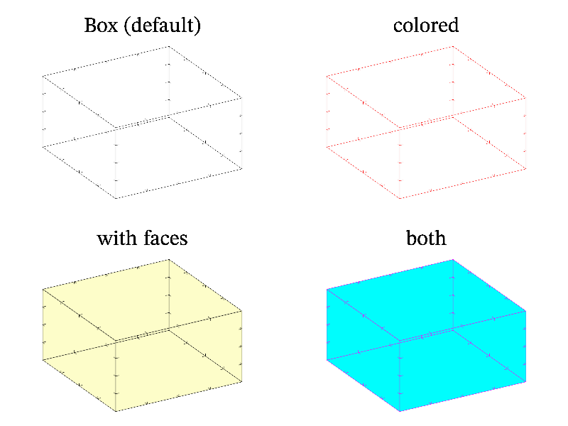
Next: Ternary axis, Previous: Colorbars, Up: Advanced usage [Contents][Index]
Box around the plot is rather useful thing because it allows one to: see the plot boundaries, and better estimate points position since box contain another set of ticks. MathGL provide special function for drawing such box – box function. By default, it draw black or white box with ticks (color depend on transparency type, see Types of transparency). However, you can change the color of box, or add drawing of rectangles at rear faces of box. Also you can disable ticks drawing, but I don’t know why anybody will want it. The sample code, which demonstrate box features is:
int sample(mglGraph *gr)
{
  gr->SubPlot(2,2,0); gr->Title("Box (default)"); gr->Rotate(50,60);
  gr->Box();
  gr->SubPlot(2,2,1); gr->Title("colored");   gr->Rotate(50,60);
  gr->Box("r");
  gr->SubPlot(2,2,2); gr->Title("with faces");  gr->Rotate(50,60);
  gr->Box("@");
  gr->SubPlot(2,2,3); gr->Title("both");  gr->Rotate(50,60);
  gr->Box("@cm");
  return 0;
}
Next: Text features, Previous: Bounding box, Up: Advanced usage [Contents][Index]
There are another unusual axis types which are supported by MathGL. These are ternary and quaternary axis. Ternary axis is special axis of 3 coordinates a, b, c which satisfy relation a+b+c=1. Correspondingly, quaternary axis is special axis of 4 coordinates a, b, c, d which satisfy relation a+b+c+d=1.
Generally speaking, only 2 of coordinates (3 for quaternary) are independent. So, MathGL just introduce some special transformation formulas which treat a as ‘x’, b as ‘y’ (and c as ‘z’ for quaternary). As result, all plotting functions (curves, surfaces, contours and so on) work as usual, but in new axis. You should use ternary function for switching to ternary/quaternary coordinates. The sample code is:
int sample(mglGraph *gr)
{
  gr->SetRanges(0,1,0,1,0,1);
  mglData x(50),y(50),z(50),rx(10),ry(10), a(20,30);
  a.Modify("30*x*y*(1-x-y)^2*(x+y<1)");
  x.Modify("0.25*(1+cos(2*pi*x))");
  y.Modify("0.25*(1+sin(2*pi*x))");
  rx.Modify("rnd"); ry.Modify("(1-v)*rnd",rx);
  z.Modify("x");

  gr->SubPlot(2,2,0); gr->Title("Ordinary axis 3D");
  gr->Rotate(50,60);    gr->Light(true);
  gr->Plot(x,y,z,"r2"); gr->Surf(a,"BbcyrR#");
  gr->Axis(); gr->Grid(); gr->Box();
  gr->Label('x',"B",1); gr->Label('y',"C",1); gr->Label('z',"Z",1);

  gr->SubPlot(2,2,1); gr->Title("Ternary axis (x+y+t=1)");
  gr->Ternary(1);
  gr->Plot(x,y,"r2"); gr->Plot(rx,ry,"q^ ");  gr->Cont(a,"BbcyrR");
  gr->Line(mglPoint(0.5,0), mglPoint(0,0.75), "g2");
  gr->Axis(); gr->Grid("xyz","B;");
  gr->Label('x',"B"); gr->Label('y',"C"); gr->Label('t',"A");

  gr->SubPlot(2,2,2); gr->Title("Quaternary axis 3D");
  gr->Rotate(50,60);    gr->Light(true);
  gr->Ternary(2);
  gr->Plot(x,y,z,"r2"); gr->Surf(a,"BbcyrR#");
  gr->Axis(); gr->Grid(); gr->Box();
  gr->Label('t',"A",1); gr->Label('x',"B",1);
  gr->Label('y',"C",1); gr->Label('z',"D",1);

  gr->SubPlot(2,2,3); gr->Title("Ternary axis 3D");
  gr->Rotate(50,60);    gr->Light(true);
  gr->Ternary(1);
  gr->Plot(x,y,z,"r2"); gr->Surf(a,"BbcyrR#");
  gr->Axis(); gr->Grid(); gr->Box();
  gr->Label('t',"A",1); gr->Label('x',"B",1);
  gr->Label('y',"C",1); gr->Label('z',"Z",1);
  return 0;
}

Next: Legend sample, Previous: Ternary axis, Up: Advanced usage [Contents][Index]
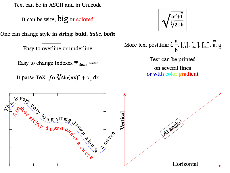
MathGL prints text by vector font. There are functions for manual specifying of text position (like Puts) and for its automatic selection (like Label, Legend and so on). MathGL prints text always in specified position even if it lies outside the bounding box. The default size of font is specified by functions SetFontSize* (see Font settings). However, the actual size of output string depends on subplot size (depends on functions SubPlot, InPlot). The switching of the font style (italic, bold, wire and so on) can be done for the whole string (by function parameter) or inside the string. By default MathGL parses TeX-like commands for symbols and indexes (see Font styles).
Text can be printed as usual one (from left to right), along some direction (rotated text), or along a curve. Text can be printed on several lines, divided by new line symbol ‘\n’.
Example of MathGL font drawing is:
int sample(mglGraph *gr)
{
  gr->SubPlot(2,2,0,"");
  gr->Putsw(mglPoint(0,1),L"Text can be in ASCII and in Unicode");
  gr->Puts(mglPoint(0,0.6),"It can be \\wire{wire}, \\big{big} or #r{colored}");
  gr->Puts(mglPoint(0,0.2),"One can change style in string: "
  "\\b{bold}, \\i{italic, \\b{both}}");
  gr->Puts(mglPoint(0,-0.2),"Easy to \\a{overline} or "
  "\\u{underline}");
  gr->Puts(mglPoint(0,-0.6),"Easy to change indexes ^{up} _{down} @{center}");
  gr->Puts(mglPoint(0,-1),"It parse TeX: \\int \\alpha \\cdot "
  "\\sqrt3{sin(\\pi x)^2 + \\gamma_{i_k}} dx");

  gr->SubPlot(2,2,1,"");
  gr->Puts(mglPoint(0,0.5), "\\sqrt{\\frac{\\alpha^{\\gamma^2}+\\overset 1{\\big\\infty}}{\\sqrt3{2+b}}}", "@", -4);
  gr->Puts(mglPoint(0,-0.5),"Text can be printed\non several lines");

  gr->SubPlot(2,2,2,"");
  mglData y;  mgls_prepare1d(&y);
  gr->Box();  gr->Plot(y.SubData(-1,0));
  gr->Text(y,"This is very very long string drawn along a curve",":k");
  gr->Text(y,"Another string drawn under a curve","T:r");

  gr->SubPlot(2,2,3,"");
  gr->Line(mglPoint(-1,-1),mglPoint(1,-1),"rA");
  gr->Puts(mglPoint(0,-1),mglPoint(1,-1),"Horizontal");
  gr->Line(mglPoint(-1,-1),mglPoint(1,1),"rA");
  gr->Puts(mglPoint(0,0),mglPoint(1,1),"At angle","@");
  gr->Line(mglPoint(-1,-1),mglPoint(-1,1),"rA");
  gr->Puts(mglPoint(-1,0),mglPoint(-1,1),"Vertical");
  return 0;
}
You can change font faces by loading font files by function loadfont. Note, that this is long-run procedure. Font faces can be downloaded from MathGL website or from here. The sample code is:
int sample(mglGraph *gr)
{
  double h=1.1, d=0.25;
  gr->LoadFont("STIX");     gr->Puts(mglPoint(0,h), "default font (STIX)");
  gr->LoadFont("adventor"); gr->Puts(mglPoint(0,h-d), "adventor font");
  gr->LoadFont("bonum");    gr->Puts(mglPoint(0,h-2*d), "bonum font");
  gr->LoadFont("chorus");   gr->Puts(mglPoint(0,h-3*d), "chorus font");
  gr->LoadFont("cursor");   gr->Puts(mglPoint(0,h-4*d), "cursor font");
  gr->LoadFont("heros");    gr->Puts(mglPoint(0,h-5*d), "heros font");
  gr->LoadFont("heroscn");  gr->Puts(mglPoint(0,h-6*d), "heroscn font");
  gr->LoadFont("pagella");  gr->Puts(mglPoint(0,h-7*d), "pagella font");
  gr->LoadFont("schola");   gr->Puts(mglPoint(0,h-8*d), "schola font");
  gr->LoadFont("termes");   gr->Puts(mglPoint(0,h-9*d), "termes font");
  return 0;
}

Next: Cutting sample, Previous: Text features, Up: Advanced usage [Contents][Index]
Legend is one of standard ways to show plot annotations. Basically you need to connect the plot style (line style, marker and color) with some text. In MathGL, you can do it by 2 methods: manually using addlegend function; or use ‘legend’ option (see Command options), which will use last plot style. In both cases, legend entries will be added into internal accumulator, which later used for legend drawing itself. clearlegend function allow you to remove all saved legend entries.
There are 2 features. If plot style is empty then text will be printed without indent. If you want to plot the text with indent but without plot sample then you need to use space ‘ ’ as plot style. Such style ‘ ’ will draw a plot sample (line with marker(s)) which is invisible line (i.e. nothing) and print the text with indent as usual one.
Function legend draw legend on the plot. The position of the legend can be selected automatic or manually. You can change the size and style of text labels, as well as setup the plot sample. The sample code demonstrating legend features is:
int sample(mglGraph *gr)
{
  gr->AddLegend("sin(\\pi {x^2})","b");
  gr->AddLegend("sin(\\pi x)","g*");
  gr->AddLegend("sin(\\pi \\sqrt{x})","rd");
  gr->AddLegend("just text"," ");
  gr->AddLegend("no indent for this","");

  gr->SubPlot(2,2,0,""); gr->Title("Legend (default)");
  gr->Box();  gr->Legend();

  gr->Legend(3,"A#");
  gr->Puts(mglPoint(0.75,0.65),"Absolute position","A");

  gr->SubPlot(2,2,2,"");  gr->Title("coloring");  gr->Box();
  gr->Legend(0,"r#"); gr->Legend(1,"Wb#");  gr->Legend(2,"ygr#");

  gr->SubPlot(2,2,3,"");  gr->Title("manual position"); gr->Box();
  gr->Legend(0.5,1);  gr->Puts(mglPoint(0.5,0.55),"at x=0.5, y=1","a");
  gr->Legend(1,"#-"); gr->Puts(mglPoint(0.75,0.25),"Horizontal legend","a");
  return 0;
}

Previous: Legend sample, Up: Advanced usage [Contents][Index]
The last common thing which I want to show in this section is how one can cut off points from plot. There are 4 mechanism for that.
SetCut function. As result all points out of bounding box will be omitted.
SetCutBox function. All points inside this box will be omitted.
SetCutOff function. All points for which the value of formula is nonzero will be omitted. Note, that this is the slowest variant.
Below I place the code which demonstrate last 3 possibilities:
int sample(mglGraph *gr)
{
  mglData a,c,v(1); mgls_prepare2d(&a); mgls_prepare3d(&c); v.a[0]=0.5;
  gr->SubPlot(2,2,0); gr->Title("Cut on (default)");
  gr->Rotate(50,60);  gr->Light(true);
  gr->Box();  gr->Surf(a,"","zrange -1 0.5");

  gr->SubPlot(2,2,1); gr->Title("Cut off");   gr->Rotate(50,60);
  gr->Box();  gr->Surf(a,"","zrange -1 0.5; cut off");

  gr->SubPlot(2,2,2); gr->Title("Cut in box");  gr->Rotate(50,60);
  gr->SetCutBox(mglPoint(0,-1,-1), mglPoint(1,0,1.1));
  gr->Alpha(true);  gr->Box();  gr->Surf3(c);
  gr->SetCutBox(mglPoint(0), mglPoint(0));  // switch it off

  gr->SubPlot(2,2,3); gr->Title("Cut by formula");  gr->Rotate(50,60);
  gr->CutOff("(z>(x+0.5*y-1)^2-1) & (z>(x-0.5*y-1)^2-1)");
  gr->Box();  gr->Surf3(c); gr->CutOff(""); // switch it off
  return 0;
}

Next: Data plotting, Previous: Advanced usage, Up: Examples [Contents][Index]
Class mglData contains all functions for the data handling in MathGL (see Data processing). There are several matters why I use class mglData but not a single array: it does not depend on type of data (mreal or double), sizes of data arrays are kept with data, memory working is simpler and safer.
| • Array creation | ||
| • Linking array | ||
| • Change data |
Next: Linking array, Up: Data handling [Contents][Index]
There are many ways in MathGL how data arrays can be created and filled.
One can put the data in mglData instance by several ways. Let us do it for sinus function:
mglData variable
  double *a = new double[50];
  for(int i=0;i<50;i++)   a[i] = sin(M_PI*i/49.);

  mglData y;
  y.Set(a,50);
mglData instance of the desired size and then to work directly with data in this variable
  mglData y(50);
  for(int i=0;i<50;i++)   y.a[i] = sin(M_PI*i/49.);
mglData instance by textual formula with the help of Modify() function
  mglData y(50);
  y.Modify("sin(pi*x)");
  mglData y(50);
  y.Fill(0,M_PI);
  y.Modify("sin(u)");
  FILE *fp=fopen("sin.dat","wt");   // create file first
  for(int i=0;i<50;i++)   fprintf(fp,"%g\n",sin(M_PI*i/49.));
  fclose(fp);

  mglData y("sin.dat");             // load it
At this you can use textual or HDF files, as well as import values from bitmap image (PNG is supported right now).
  FILE *fp-fopen("sin.dat","wt");   // create large file first
  for(int i=0;i<70;i++)   fprintf(fp,"%g\n",sin(M_PI*i/49.));
  fclose(fp);

  mglData y;
  y.Read("sin.dat",50);             // load it
Creation of 2d- and 3d-arrays is mostly the same. But one should keep in mind that class mglData uses flat data representation. For example, matrix 30*40 is presented as flat (1d-) array with length 30*40=1200 (nx=30, ny=40). The element with indexes {i,j} is a[i+nx*j]. So for 2d array we have:
  mglData z(30,40);
  for(int i=0;i<30;i++)   for(int j=0;j<40;j++)
    z.a[i+30*j] = sin(M_PI*i/29.)*sin(M_PI*j/39.);
or by using Modify() function
  mglData z(30,40);
  z.Modify("sin(pi*x)*cos(pi*y)");
The only non-obvious thing here is using multidimensional arrays in C/C++, i.e. arrays defined like mreal dat[40][30];. Since, formally these elements dat[i] can address the memory in arbitrary place you should use the proper function to convert such arrays to mglData object. For C++ this is functions like mglData::Set(mreal **dat, int N1, int N2);. For C this is functions like mgl_data_set_mreal2(HMDT d, const mreal **dat, int N1, int N2);. At this, you should keep in mind that nx=N2 and ny=N1 after conversion.
Next: Change data, Previous: Array creation, Up: Data handling [Contents][Index]
Sometimes the data arrays are so large, that one couldn’t’ copy its values to another array (i.e. into mglData). In this case, he can define its own class derived from mglDataA (see mglDataA class) or can use Link function.
In last case, MathGL just save the link to an external data array, but not copy it. You should provide the existence of this data array for whole time during which MathGL can use it. Another point is that MathGL will automatically create new array if you’ll try to modify data values by any of mglData functions. So, you should use only function with const modifier if you want still using link to the original data array.
Creating the link is rather simple – just the same as using Set function
  double *a = new double[50];
  for(int i=0;i<50;i++)   a[i] = sin(M_PI*i/49.);

  mglData y;
  y.Link(a,50);
Previous: Linking array, Up: Data handling [Contents][Index]
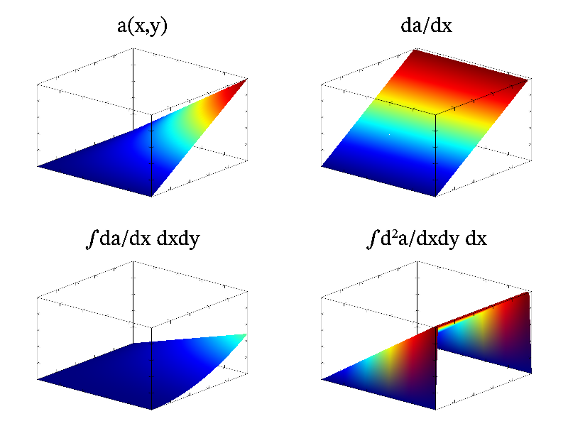
MathGL has functions for data processing: differentiating, integrating, smoothing and so on (for more detail, see Data processing). Let us consider some examples. The simplest ones are integration and differentiation. The direction in which operation will be performed is specified by textual string, which may contain symbols ‘x’, ‘y’ or ‘z’. For example, the call of Diff("x") will differentiate data along ‘x’ direction; the call of Integral("xy") perform the double integration of data along ‘x’ and ‘y’ directions; the call of Diff2("xyz") will apply 3d Laplace operator to data and so on. Example of this operations on 2d array a=x*y is presented in code:
int sample(mglGraph *gr)
{
  gr->SetRanges(0,1,0,1,0,1);
  mglData a(30,40); a.Modify("x*y");
  gr->SubPlot(2,2,0); gr->Rotate(60,40);
  gr->Surf(a);    gr->Box();
  gr->Puts(mglPoint(0.7,1,1.2),"a(x,y)");
  gr->SubPlot(2,2,1); gr->Rotate(60,40);
  a.Diff("x");    gr->Surf(a);  gr->Box();
  gr->Puts(mglPoint(0.7,1,1.2),"da/dx");
  gr->SubPlot(2,2,2); gr->Rotate(60,40);
  a.Integral("xy"); gr->Surf(a);  gr->Box();
  gr->Puts(mglPoint(0.7,1,1.2),"\\int da/dx dxdy");
  gr->SubPlot(2,2,3); gr->Rotate(60,40);
  a.Diff2("y"); gr->Surf(a);  gr->Box();
  gr->Puts(mglPoint(0.7,1,1.2),"\\int {d^2}a/dxdy dx");
  return 0;
}
Data smoothing (function smooth) is more interesting and important. This function has single argument which define type of smoothing and its direction. Now 3 methods are supported: ‘3’ – linear averaging by 3 points, ‘5’ – linear averaging by 5 points, and default one – quadratic averaging by 5 points.
MathGL also have some amazing functions which is not so important for data processing as useful for data plotting. There are functions for finding envelope (useful for plotting rapidly oscillating data), for data sewing (useful to removing jumps on the phase), for data resizing (interpolation). Let me demonstrate it:
int sample(mglGraph *gr)
{
  gr->SubPlot(2,2,0,"");  gr->Title("Envelop sample");
  mglData d1(1000); gr->Fill(d1,"exp(-8*x^2)*sin(10*pi*x)");
  gr->Axis();     gr->Plot(d1, "b");
  d1.Envelop('x');  gr->Plot(d1, "r");

  gr->SubPlot(2,2,1,"");  gr->Title("Smooth sample");
  mglData y0(30),y1,y2,y3;
  gr->SetRanges(0,1,0,1);
  gr->Fill(y0, "0.4*sin(pi*x) + 0.3*cos(1.5*pi*x) - 0.4*sin(2*pi*x)+0.5*rnd");

  y1=y0;  y1.Smooth("x3");
  y2=y0;  y2.Smooth("x5");
  y3=y0;  y3.Smooth("x");

  gr->Plot(y0,"{m7}:s", "legend 'none'"); //gr->AddLegend("none","k");
  gr->Plot(y1,"r", "legend ''3' style'");
  gr->Plot(y2,"g", "legend ''5' style'");
  gr->Plot(y3,"b", "legend 'default'");
  gr->Legend();   gr->Box();

  gr->SubPlot(2,2,2);   gr->Title("Sew sample");
  mglData d2(100, 100); gr->Fill(d2, "mod((y^2-(1-x)^2)/2,0.1)");
  gr->Rotate(50, 60);   gr->Light(true);  gr->Alpha(true);
  gr->Box();            gr->Surf(d2, "b");
  d2.Sew("xy", 0.1);  gr->Surf(d2, "r");

  gr->SubPlot(2,2,3);   gr->Title("Resize sample (interpolation)");
  mglData x0(10), v0(10), x1, v1;
  gr->Fill(x0,"rnd");     gr->Fill(v0,"rnd");
  x1 = x0.Resize(100);    v1 = v0.Resize(100);
  gr->Plot(x0,v0,"b+ ");  gr->Plot(x1,v1,"r-");
  gr->Label(x0,v0,"%n");
  return 0;
}

Also one can create new data arrays on base of the existing one: extract slice, row or column of data (subdata), summarize along a direction(s) (sum), find distribution of data elements (hist) and so on.
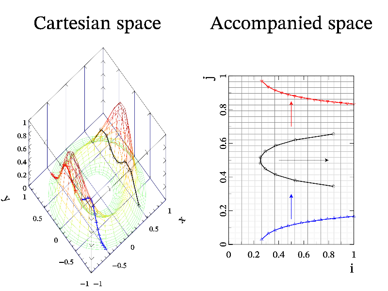
Another interesting feature of MathGL is interpolation and root-finding. There are several functions for linear and cubic spline interpolation (see Interpolation). Also there is a function evaluate which do interpolation of data array for values of each data element of index data. It look as indirect access to the data elements.
This function have inverse function solve which find array of indexes at which data array is equal to given value (i.e. work as root finding). But solve function have the issue – usually multidimensional data (2d and 3d ones) have an infinite number of indexes which give some value. This is contour lines for 2d data, or isosurface(s) for 3d data. So, solve function will return index only in given direction, assuming that other index(es) are the same as equidistant index(es) of original data. If data have multiple roots then second (and later) branches can be found by consecutive call(s) of solve function. Let me demonstrate this on the following sample.
int sample(mglGraph *gr)
{
  gr->SetRange('z',0,1);
  mglData x(20,30), y(20,30), z(20,30), xx,yy,zz;
  gr->Fill(x,"(x+2)/3*cos(pi*y)");
  gr->Fill(y,"(x+2)/3*sin(pi*y)");
  gr->Fill(z,"exp(-6*x^2-2*sin(pi*y)^2)");

  gr->SubPlot(2,1,0); gr->Title("Cartesian space");   gr->Rotate(30,-40);
  gr->Axis("xyzU");   gr->Box();  gr->Label('x',"x"); gr->Label('y',"y");
  gr->SetOrigin(1,1); gr->Grid("xy");
  gr->Mesh(x,y,z);

  // section along 'x' direction
  mglData u = x.Solve(0.5,'x');
  mglData v(u.nx);  v.Fill(0,1);
  xx = x.Evaluate(u,v);   yy = y.Evaluate(u,v);   zz = z.Evaluate(u,v);
  gr->Plot(xx,yy,zz,"k2o");

  // 1st section along 'y' direction
  mglData u1 = x.Solve(-0.5,'y');
  mglData v1(u1.nx);  v1.Fill(0,1);
  xx = x.Evaluate(v1,u1); yy = y.Evaluate(v1,u1); zz = z.Evaluate(v1,u1);
  gr->Plot(xx,yy,zz,"b2^");

  // 2nd section along 'y' direction
  mglData u2 = x.Solve(-0.5,'y',u1);
  xx = x.Evaluate(v1,u2); yy = y.Evaluate(v1,u2); zz = z.Evaluate(v1,u2);
  gr->Plot(xx,yy,zz,"r2v");

  gr->SubPlot(2,1,1); gr->Title("Accompanied space");
  gr->SetRanges(0,1,0,1); gr->SetOrigin(0,0);
  gr->Axis(); gr->Box();  gr->Label('x',"i"); gr->Label('y',"j");
  gr->Grid(z,"h");

  gr->Plot(u,v,"k2o");    gr->Line(mglPoint(0.4,0.5),mglPoint(0.8,0.5),"kA");
  gr->Plot(v1,u1,"b2^");  gr->Line(mglPoint(0.5,0.15),mglPoint(0.5,0.3),"bA");
  gr->Plot(v1,u2,"r2v");  gr->Line(mglPoint(0.5,0.7),mglPoint(0.5,0.85),"rA");
}
Next: Hints, Previous: Data handling, Up: Examples [Contents][Index]
Let me now show how to plot the data. Next section will give much more examples for all plotting functions. Here I just show some basics. MathGL generally has 2 types of plotting functions. Simple variant requires a single data array for plotting, other data (coordinates) are considered uniformly distributed in axis range. Second variant requires data arrays for all coordinates. It allows one to plot rather complex multivalent curves and surfaces (in case of parametric dependencies). Usually each function have one textual argument for plot style and another textual argument for options (see Command options).
Note, that the call of drawing function adds something to picture but does not clear the previous plots (as it does in Matlab). Another difference from Matlab is that all setup (like transparency, lightning, axis borders and so on) must be specified before plotting functions.
Let start for plots for 1D data. Term “1D data” means that data depend on single index (parameter) like curve in parametric form {x(i),y(i),z(i)}, i=1...n. The textual argument allow you specify styles of line and marks (see Line styles). If this parameter is NULL or empty then solid line with color from palette is used (see Palette and colors).
Below I shall show the features of 1D plotting on base of plot function. Let us start from sinus plot:
int sample(mglGraph *gr)
{
  mglData y0(50); 	y0.Modify("sin(pi*(2*x-1))");
  gr->SubPlot(2,2,0);
  gr->Plot(y0);   	gr->Box();
Style of line is not specified in plot function. So MathGL uses the solid line with first color of palette (this is blue). Next subplot shows array y1 with 2 rows:
  gr->SubPlot(2,2,1);
  mglData y1(50,2);
  y1.Modify("sin(pi*2*x-pi)");
  y1.Modify("cos(pi*2*x-pi)/2",1);
  gr->Plot(y1);   	gr->Box();
As previously I did not specify the style of lines. As a result, MathGL again uses solid line with next colors in palette (there are green and red). Now let us plot a circle on the same subplot. The circle is parametric curve x=cos(\pi t), y=sin(\pi t). I will set the color of the circle (dark yellow, ‘Y’) and put marks ‘+’ at point position:
  mglData x(50);  	x.Modify("cos(pi*2*x-pi)");
  gr->Plot(x,y0,"Y+");
Note that solid line is used because I did not specify the type of line. The same picture can be achieved by plot and subdata functions. Let us draw ellipse by orange dash line:
gr->Plot(y1.SubData(-1,0),y1.SubData(-1,1),"q|");
Drawing in 3D space is mostly the same. Let us draw spiral with default line style. Now its color is 4-th color from palette (this is cyan):
  gr->SubPlot(2,2,2);	gr->Rotate(60,40);
  mglData z(50);  	z.Modify("2*x-1");
  gr->Plot(x,y0,z);	gr->Box();
Functions plot and subdata make 3D curve plot but for single array. Use it to put circle marks on the previous plot:
  mglData y2(10,3);	y2.Modify("cos(pi*(2*x-1+y))");
  y2.Modify("2*x-1",2);
  gr->Plot(y2.SubData(-1,0),y2.SubData(-1,1),y2.SubData(-1,2),"bo ");
Note that line style is empty ‘ ’ here. Usage of other 1D plotting functions looks similar:
  gr->SubPlot(2,2,3);	gr->Rotate(60,40);
  gr->Bars(x,y0,z,"r");	gr->Box();
  return 0;
}
Surfaces surf and other 2D plots (see 2D plotting) are drown the same simpler as 1D one. The difference is that the string parameter specifies not the line style but the color scheme of the plot (see Color scheme). Here I draw attention on 4 most interesting color schemes. There is gray scheme where color is changed from black to white (string ‘kw’) or from white to black (string ‘wk’). Another scheme is useful for accentuation of negative (by blue color) and positive (by red color) regions on plot (string ‘"BbwrR"’). Last one is the popular “jet” scheme (string ‘"BbcyrR"’).
Now I shall show the example of a surface drawing. At first let us switch lightning on
int sample(mglGraph *gr)
{
  gr->Light(true);	gr->Light(0,mglPoint(0,0,1));
and draw the surface, considering coordinates x,y to be uniformly distributed in axis range
  mglData a0(50,40);
  a0.Modify("0.6*sin(2*pi*x)*sin(3*pi*y)+0.4*cos(3*pi*(x*y))");
  gr->SubPlot(2,2,0);	gr->Rotate(60,40);
  gr->Surf(a0);		gr->Box();
Color scheme was not specified. So previous color scheme is used. In this case it is default color scheme (“jet”) for the first plot. Next example is a sphere. The sphere is parametrically specified surface:
  mglData x(50,40),y(50,40),z(50,40);
  x.Modify("0.8*sin(2*pi*x)*sin(pi*y)");
  y.Modify("0.8*cos(2*pi*x)*sin(pi*y)");
  z.Modify("0.8*cos(pi*y)");
  gr->SubPlot(2,2,1);	gr->Rotate(60,40);
  gr->Surf(x,y,z,"BbwrR");gr->Box();
I set color scheme to "BbwrR" that corresponds to red top and blue bottom of the sphere.
Surfaces will be plotted for each of slice of the data if nz>1. Next example draws surfaces for data arrays with nz=3:
  mglData a1(50,40,3);
  a1.Modify("0.6*sin(2*pi*x)*sin(3*pi*y)+0.4*cos(3*pi*(x*y))");
  a1.Modify("0.6*cos(2*pi*x)*cos(3*pi*y)+0.4*sin(3*pi*(x*y))",1);
  a1.Modify("0.6*cos(2*pi*x)*cos(3*pi*y)+0.4*cos(3*pi*(x*y))",2);
  gr->SubPlot(2,2,2);	gr->Rotate(60,40);
  gr->Alpha(true);
  gr->Surf(a1);		gr->Box();
Note, that it may entail a confusion. However, if one will use density plot then the picture will look better:
  gr->SubPlot(2,2,3);	gr->Rotate(60,40);
  gr->Dens(a1);		gr->Box();
  return 0;
}
Drawing of other 2D plots is analogous. The only peculiarity is the usage of flag ‘#’. By default this flag switches on the drawing of a grid on plot (grid or mesh for plots in plain or in volume). However, for isosurfaces (including surfaces of rotation axial) this flag switches the face drawing off and figure becomes wired. The following code gives example of flag ‘#’ using (compare with normal function drawing as in its description):
int sample(mglGraph *gr)
{
  gr->Alpha(true);	gr->Light(true);	gr->Light(0,mglPoint(0,0,1));
  mglData a(30,20);
  a.Modify("0.6*sin(2*pi*x)*sin(3*pi*y) + 0.4*cos(3*pi*(x*y))");

  gr->SubPlot(2,2,0);	gr->Rotate(40,60);
  gr->Surf(a,"BbcyrR#");		gr->Box();
  gr->SubPlot(2,2,1);	gr->Rotate(40,60);
  gr->Dens(a,"BbcyrR#");		gr->Box();
  gr->SubPlot(2,2,2);	gr->Rotate(40,60);
  gr->Cont(a,"BbcyrR#");		gr->Box();
  gr->SubPlot(2,2,3);	gr->Rotate(40,60);
  gr->Axial(a,"BbcyrR#");		gr->Box();
  return 0;
}
Next: FAQ, Previous: Data plotting, Up: Examples [Contents][Index]
In this section I’ve included some small hints and advices for the improving of the quality of plots and for the demonstration of some non-trivial features of MathGL library. In contrast to previous examples I showed mostly the idea but not the whole drawing function.
Next: Transparency and lighting, Up: Hints [Contents][Index]
As I noted above, MathGL functions (except the special one, like Clf()) do not erase the previous plotting but just add the new one. It allows one to draw “compound” plots easily. For example, popular Matlab command surfc can be emulated in MathGL by 2 calls:
  Surf(a);
  Cont(a, "_");     // draw contours at bottom
Here a is 2-dimensional data for the plotting, -1 is the value of z-coordinate at which the contour should be plotted (at the bottom in this example). Analogously, one can draw density plot instead of contour lines and so on.
Another nice plot is contour lines plotted directly on the surface:
  Light(true);       // switch on light for the surface
  Surf(a, "BbcyrR"); // select 'jet' colormap for the surface
  Cont(a, "y");      // and yellow color for contours
The possible difficulties arise in black&white case, when the color of the surface can be close to the color of a contour line. In that case I may suggest the following code:
  Light(true);   // switch on light for the surface
  Surf(a, "kw"); // select 'gray' colormap for the surface
  CAxis(-1,0);   // first draw for darker surface colors
  Cont(a, "w");  // white contours
  CAxis(0,1);    // now draw for brighter surface colors
  Cont(a, "k");  // black contours
  CAxis(-1,1);   // return color range to original state
The idea is to divide the color range on 2 parts (dark and bright) and to select the contrasting color for contour lines for each of part.
Similarly, one can plot flow thread over density plot of vector field amplitude (this is another amusing plot from Matlab) and so on. The list of compound graphics can be prolonged but I hope that the general idea is clear.
Just for illustration I put here following sample code:
int sample(mglGraph *gr)
{
  mglData a,b,d;  mgls_prepare2v(&a,&b);  d = a;
  for(int i=0;i<a.nx*a.ny;i++)  d.a[i] = hypot(a.a[i],b.a[i]);
  mglData c;  mgls_prepare3d(&c);
  mglData v(10);  v.Fill(-0.5,1);

  gr->SubPlot(2,2,1,"");  gr->Title("Flow + Dens");
  gr->Flow(a,b,"br"); gr->Dens(d,"BbcyrR"); gr->Box();

  gr->SubPlot(2,2,0); gr->Title("Surf + Cont"); gr->Rotate(50,60);
  gr->Light(true);  gr->Surf(a);  gr->Cont(a,"y");  gr->Box();

  gr->SubPlot(2,2,2); gr->Title("Mesh + Cont"); gr->Rotate(50,60);
  gr->Box();  gr->Mesh(a);  gr->Cont(a,"_");

  gr->SubPlot(2,2,3); gr->Title("Surf3 + ContF3");gr->Rotate(50,60);
  gr->Box();  gr->ContF3(v,c,"z",0);  gr->ContF3(v,c,"x");  gr->ContF3(v,c);
  gr->SetCutBox(mglPoint(0,-1,-1), mglPoint(1,0,1.1));
  gr->ContF3(v,c,"z",c.nz-1); gr->Surf3(-0.5,c);
  return 0;
}

Next: Types of transparency, Previous: ``Compound'' graphics, Up: Hints [Contents][Index]
Here I want to show how transparency and lighting both and separately change the look of a surface. So, there is code and picture for that:
int sample(mglGraph *gr)
{
  mglData a;  mgls_prepare2d(&a);
  gr->SubPlot(2,2,0); gr->Title("default"); gr->Rotate(50,60);
  gr->Box();  gr->Surf(a);

  gr->SubPlot(2,2,1); gr->Title("light on");  gr->Rotate(50,60);
  gr->Box();  gr->Light(true);  gr->Surf(a);

  gr->SubPlot(2,2,3); gr->Title("alpha on; light on");  gr->Rotate(50,60);
  gr->Box();  gr->Alpha(true);  gr->Surf(a);

  gr->SubPlot(2,2,2); gr->Title("alpha on");  gr->Rotate(50,60);
  gr->Box();  gr->Light(false); gr->Surf(a);
  return 0;
}
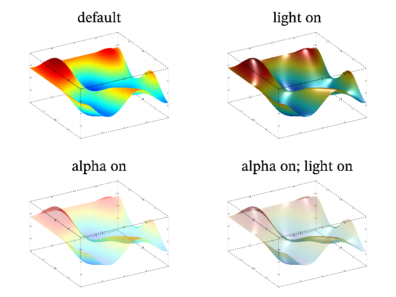
Next: Axis projection, Previous: Transparency and lighting, Up: Hints [Contents][Index]
MathGL library has advanced features for setting and handling the surface transparency. The simplest way to add transparency is the using of function alpha. As a result, all further surfaces (and isosurfaces, density plots and so on) become transparent. However, their look can be additionally improved.
The value of transparency can be different from surface to surface. To do it just use SetAlphaDef before the drawing of the surface, or use option alpha (see Command options). If its value is close to 0 then the surface becomes more and more transparent. Contrary, if its value is close to 1 then the surface becomes practically non-transparent.
Also you can change the way how the light goes through overlapped surfaces. The function SetTranspType defines it. By default the usual transparency is used (‘0’) – surfaces below is less visible than the upper ones. A “glass-like” transparency (‘1’) has a different look – each surface just decreases the background light (the surfaces are commutable in this case).
A “neon-like” transparency (‘2’) has more interesting look. In this case a surface is the light source (like a lamp on the dark background) and just adds some intensity to the color. At this, the library sets automatically the black color for the background and changes the default line color to white.
As example I shall show several plots for different types of transparency. The code is the same except the values of SetTranspType function:
int sample(mglGraph *gr)
{
  gr->Alpha(true);  gr->Light(true);
  mglData a;  mgls_prepare2d(&a);
  gr->SetTranspType(0); gr->Clf();
  gr->SubPlot(2,2,0); gr->Rotate(50,60);  gr->Surf(a);  gr->Box();
  gr->SubPlot(2,2,1); gr->Rotate(50,60);  gr->Dens(a);  gr->Box();
  gr->SubPlot(2,2,2); gr->Rotate(50,60);  gr->Cont(a);  gr->Box();
  gr->SubPlot(2,2,3); gr->Rotate(50,60);  gr->Axial(a); gr->Box();
  return 0;
}
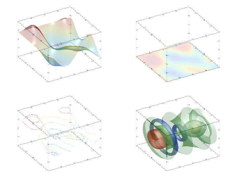
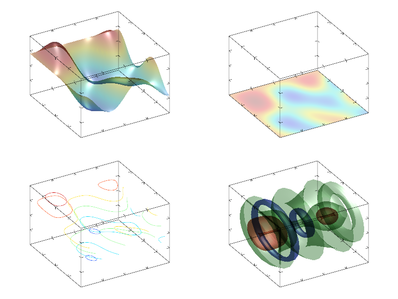
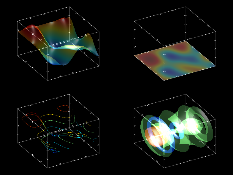
Next: Adding fog, Previous: Types of transparency, Up: Hints [Contents][Index]
You can easily make 3D plot and draw its x-,y-,z-projections (like in CAD) by using ternary function with arguments: 4 for Cartesian, 5 for Ternary and 6 for Quaternary coordinates. The sample code is:
int sample(mglGraph *gr)
{
  gr->SetRanges(0,1,0,1,0,1);
  mglData x(50),y(50),z(50),rx(10),ry(10), a(20,30);
  a.Modify("30*x*y*(1-x-y)^2*(x+y<1)");
  x.Modify("0.25*(1+cos(2*pi*x))");
  y.Modify("0.25*(1+sin(2*pi*x))");
  rx.Modify("rnd"); ry.Modify("(1-v)*rnd",rx);
  z.Modify("x");

  gr->Title("Projection sample");
  gr->Ternary(4);
  gr->Rotate(50,60);      gr->Light(true);
  gr->Plot(x,y,z,"r2");   gr->Surf(a,"#");
  gr->Axis(); gr->Grid(); gr->Box();
  gr->Label('x',"X",1);   gr->Label('y',"Y",1);   gr->Label('z',"Z",1);
}
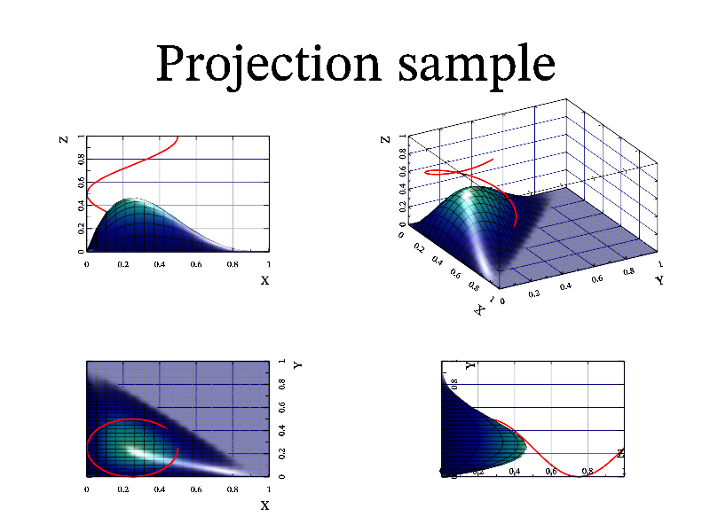
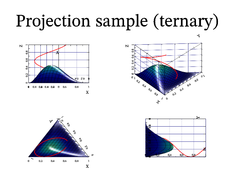
Next: Lighting sample, Previous: Axis projection, Up: Hints [Contents][Index]
MathGL can add a fog to the image. Its switching on is rather simple – just use fog function. There is the only feature – fog is applied for whole image. Not to particular subplot. The sample code is:
int sample(mglGraph *gr)
{
  mglData a;  mgls_prepare2d(&a);
  gr->Title("Fog sample");
  gr->Light(true);  gr->Rotate(50,60);  gr->Fog(1); gr->Box();
  gr->Surf(a);  gr->Cont(a,"y");
  return 0;
}
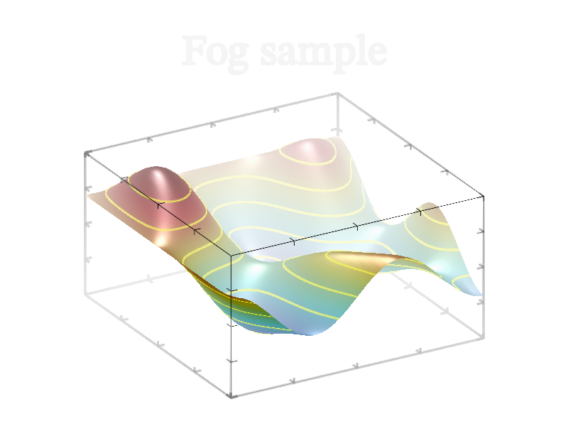
Next: Using primitives, Previous: Adding fog, Up: Hints [Contents][Index]
In contrast to the most of other programs, MathGL supports several (up to 10) light sources. Moreover, the color each of them can be different: white (this is usual), yellow, red, cyan, green and so on. The use of several light sources may be interesting for the highlighting of some peculiarities of the plot or just to make an amusing picture. Note, each light source can be switched on/off individually. The sample code is:
int sample(mglGraph *gr)
{
  mglData a;  mgls_prepare2d(&a);
  gr->Title("Several light sources");
  gr->Rotate(50,60);  gr->Light(true);
  gr->AddLight(1,mglPoint(0,1,0),'c');
  gr->AddLight(2,mglPoint(1,0,0),'y');
  gr->AddLight(3,mglPoint(0,-1,0),'m');
  gr->Box();  gr->Surf(a,"h");
  return 0;
}
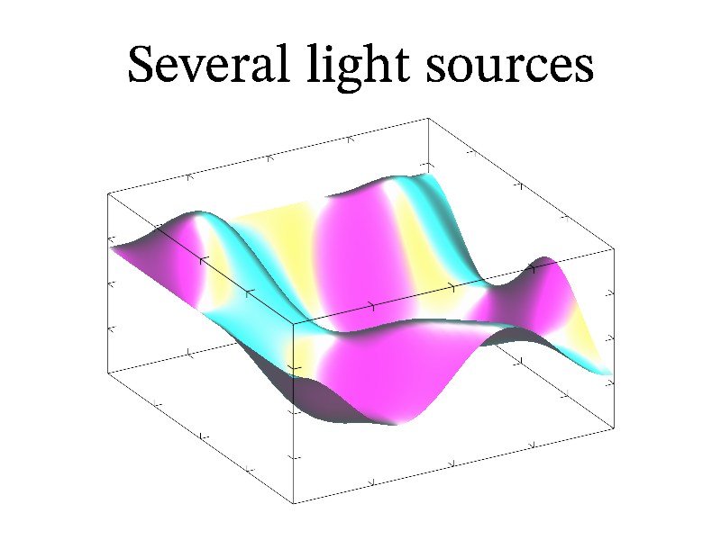
Additionally, you can use local light sources and set to use diffuse reflection instead of specular one (by default) or both kinds. Note, I use attachlight command to keep light settings relative to subplot.
int sample(mglGraph *gr)
{
  gr->Light(true);  gr->AttachLight(true);
  gr->SubPlot(2,2,0); gr->Title("Default"); gr->Rotate(50,60);
  gr->Line(mglPoint(-1,-0.7,1.7),mglPoint(-1,-0.7,0.7),"BA"); gr->Box();  gr->Surf(a);

  gr->SubPlot(2,2,1); gr->Title("Local");   gr->Rotate(50,60);
  gr->AddLight(0,mglPoint(1,0,1),mglPoint(-2,-1,-1));
  gr->Line(mglPoint(1,0,1),mglPoint(-1,-1,0),"BAO");  gr->Box();  gr->Surf(a);

  gr->SubPlot(2,2,2); gr->Title("no diffuse"); gr->Rotate(50,60);
  gr->SetDiffuse(0);
  gr->Line(mglPoint(1,0,1),mglPoint(-1,-1,0),"BAO");  gr->Box();  gr->Surf(a);

  gr->SubPlot(2,2,3); gr->Title("diffusive only");  gr->Rotate(50,60);
  gr->SetDiffuse(0.5);
  gr->AddLight(0,mglPoint(1,0,1),mglPoint(-2,-1,-1),'w',0);
  gr->Line(mglPoint(1,0,1),mglPoint(-1,-1,0),"BAO");  gr->Box();  gr->Surf(a);
}
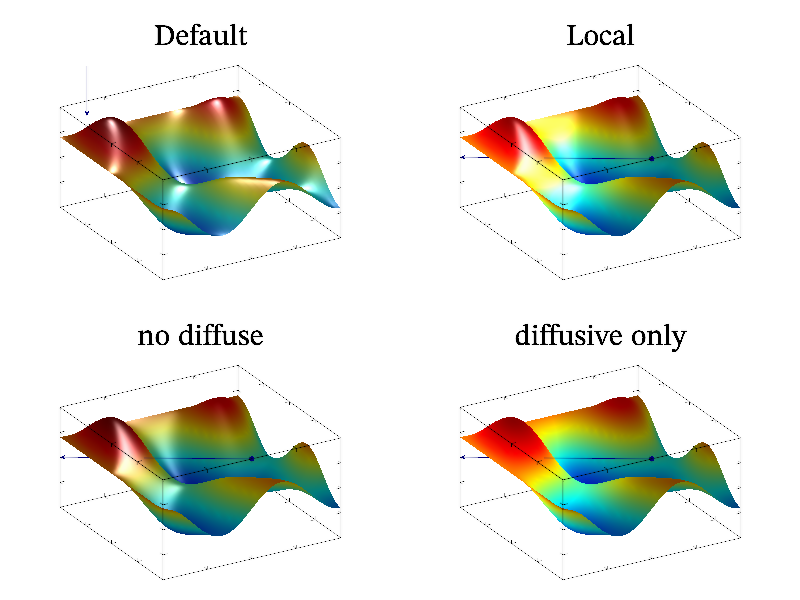
Next: STFA sample, Previous: Lighting sample, Up: Hints [Contents][Index]
MathGL provide a set of functions for drawing primitives (see Primitives). Primitives are low level object, which used by most of plotting functions. Picture below demonstrate some of commonly used primitives.

Generally, you can create arbitrary new kind of plot using primitives. For example, MathGL don’t provide any special functions for drawing molecules. However, you can do it using only one type of primitives drop. The sample code is:
int sample(mglGraph *gr)
{
  gr->Alpha(true);  gr->Light(true);

  gr->SubPlot(2,2,0,"");  gr->Title("Methane, CH_4");
  gr->StartGroup("Methane");
  gr->Rotate(60,120);
  gr->Sphere(mglPoint(0,0,0),0.25,"k");
  gr->Drop(mglPoint(0,0,0),mglPoint(0,0,1),0.35,"h",1,2);
  gr->Sphere(mglPoint(0,0,0.7),0.25,"g");
  gr->Drop(mglPoint(0,0,0),mglPoint(-0.94,0,-0.33),0.35,"h",1,2);
  gr->Sphere(mglPoint(-0.66,0,-0.23),0.25,"g");
  gr->Drop(mglPoint(0,0,0),mglPoint(0.47,0.82,-0.33),0.35,"h",1,2);
  gr->Sphere(mglPoint(0.33,0.57,-0.23),0.25,"g");
  gr->Drop(mglPoint(0,0,0),mglPoint(0.47,-0.82,-0.33),0.35,"h",1,2);
  gr->Sphere(mglPoint(0.33,-0.57,-0.23),0.25,"g");
  gr->EndGroup();

  gr->SubPlot(2,2,1,"");  gr->Title("Water, H_{2}O");
  gr->StartGroup("Water");
  gr->Rotate(60,100);
  gr->StartGroup("Water_O");
  gr->Sphere(mglPoint(0,0,0),0.25,"r");
  gr->EndGroup();
  gr->StartGroup("Water_Bond_1");
  gr->Drop(mglPoint(0,0,0),mglPoint(0.3,0.5,0),0.3,"m",1,2);
  gr->EndGroup();
  gr->StartGroup("Water_H_1");
  gr->Sphere(mglPoint(0.3,0.5,0),0.25,"g");
  gr->EndGroup();
  gr->StartGroup("Water_Bond_2");
  gr->Drop(mglPoint(0,0,0),mglPoint(0.3,-0.5,0),0.3,"m",1,2);
  gr->EndGroup();
  gr->StartGroup("Water_H_2");
  gr->Sphere(mglPoint(0.3,-0.5,0),0.25,"g");
  gr->EndGroup();
  gr->EndGroup();

  gr->SubPlot(2,2,2,"");  gr->Title("Oxygen, O_2");
  gr->StartGroup("Oxygen");
  gr->Rotate(60,120);
  gr->Drop(mglPoint(0,0.5,0),mglPoint(0,-0.3,0),0.3,"m",1,2);
  gr->Sphere(mglPoint(0,0.5,0),0.25,"r");
  gr->Drop(mglPoint(0,-0.5,0),mglPoint(0,0.3,0),0.3,"m",1,2);
  gr->Sphere(mglPoint(0,-0.5,0),0.25,"r");
  gr->EndGroup();

  gr->SubPlot(2,2,3,"");  gr->Title("Ammonia, NH_3");
  gr->StartGroup("Ammonia");
  gr->Rotate(60,120);
  gr->Sphere(mglPoint(0,0,0),0.25,"b");
  gr->Drop(mglPoint(0,0,0),mglPoint(0.33,0.57,0),0.32,"n",1,2);
  gr->Sphere(mglPoint(0.33,0.57,0),0.25,"g");
  gr->Drop(mglPoint(0,0,0),mglPoint(0.33,-0.57,0),0.32,"n",1,2);
  gr->Sphere(mglPoint(0.33,-0.57,0),0.25,"g");
  gr->Drop(mglPoint(0,0,0),mglPoint(-0.65,0,0),0.32,"n",1,2);
  gr->Sphere(mglPoint(-0.65,0,0),0.25,"g");
  gr->EndGroup();
  return 0;
}
Moreover, some of special plots can be more easily produced by primitives rather than by specialized function. For example, Venn diagram can be produced by Error plot:
int sample(mglGraph *gr)
{
  double xx[3]={-0.3,0,0.3}, yy[3]={0.3,-0.3,0.3}, ee[3]={0.7,0.7,0.7};
  mglData x(3,xx), y(3,yy), e(3,ee);
  gr->Title("Venn-like diagram"); gr->Alpha(true);
  gr->Error(x,y,e,e,"!rgb@#o");
  return 0;
}
You see that you have to specify and fill 3 data arrays. The same picture can be produced by just 3 calls of circle function:
int sample(mglGraph *gr)
{
  gr->Title("Venn-like diagram"); gr->Alpha(true);
  gr->Circle(mglPoint(-0.3,0.3),0.7,"rr@");
  gr->Circle(mglPoint(0,-0.3),0.7,"gg@");
  gr->Circle(mglPoint( 0.3,0.3),0.7,"bb@");
  return 0;
}
Of course, the first variant is more suitable if you need to plot a lot of circles. But for few ones the usage of primitives looks easy.

Next: Mapping visualization, Previous: Using primitives, Up: Hints [Contents][Index]
Short-time Fourier Analysis (stfa) is one of informative method for analyzing long rapidly oscillating 1D data arrays. It is used to determine the sinusoidal frequency and phase content of local sections of a signal as it changes over time.
MathGL can find and draw STFA result. Just to show this feature I give following sample. Initial data arrays is 1D arrays with step-like frequency. Exactly this you can see at bottom on the STFA plot. The sample code is:
int sample(mglGraph *gr)
{
  mglData a(2000), b(2000);
  gr->Fill(a,"cos(50*pi*x)*(x<-.5)+cos(100*pi*x)*(x<0)*(x>-.5)+\
  cos(200*pi*x)*(x<.5)*(x>0)+cos(400*pi*x)*(x>.5)");
  gr->SubPlot(1, 2, 0,"<_");  gr->Title("Initial signal");
  gr->Plot(a);
  gr->Axis();
  gr->Label('x', "\\i t");

  gr->SubPlot(1, 2, 1,"<_");  gr->Title("STFA plot");
  gr->STFA(a, b, 64);
  gr->Axis();
  gr->Label('x', "\\i t");
  gr->Label('y', "\\omega", 0);
  return 0;
}
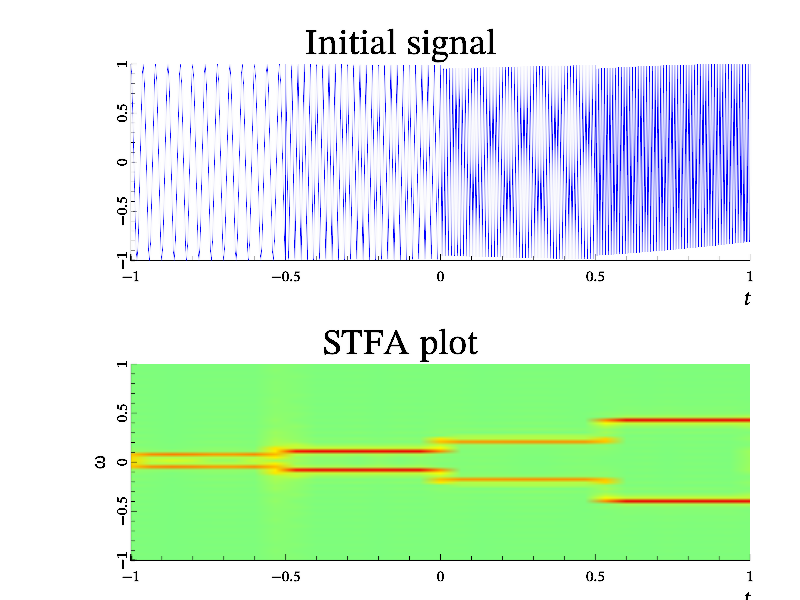
Next: Data interpolation, Previous: STFA sample, Up: Hints [Contents][Index]
Sometime ago I worked with mapping and have a question about its visualization. Let me remember you that mapping is some transformation rule for one set of number to another one. The 1d mapping is just an ordinary function – it takes a number and transforms it to another one. The 2d mapping (which I used) is a pair of functions which take 2 numbers and transform them to another 2 ones. Except general plots (like surfc, surfa) there is a special plot – Arnold diagram. It shows the area which is the result of mapping of some initial area (usually square).
I tried to make such plot in map. It shows the set of points or set of faces, which final position is the result of mapping. At this, the color gives information about their initial position and the height describes Jacobian value of the transformation. Unfortunately, it looks good only for the simplest mapping but for the real multivalent quasi-chaotic mapping it produces a confusion. So, use it if you like :).
The sample code for mapping visualization is:
int sample(mglGraph *gr)
{
  mglData a(50, 40), b(50, 40);
  gr->Puts(mglPoint(0, 0), "\\to", ":C", -1.4);
  gr->SetRanges(-1,1,-1,1,-2,2);

  gr->SubPlot(2, 1, 0);
  gr->Fill(a,"x");  gr->Fill(b,"y");
  gr->Puts(mglPoint(0, 1.1), "\\{x, y\\}", ":C", -2);   gr->Box();
  gr->Map(a, b, "brgk");

  gr->SubPlot(2, 1, 1);
  gr->Fill(a,"(x^3+y^3)/2");  gr->Fill(b,"(x-y)/2");
  gr->Puts(mglPoint(0, 1.1), "\\{\\frac{x^3+y^3}{2}, \\frac{x-y}{2}\\}", ":C", -2);
  gr->Box();
  gr->Map(a, b, "brgk");
  return 0;
}

Next: Making regular data, Previous: Mapping visualization, Up: Hints [Contents][Index]
There are many functions to get interpolated values of a data array. Basically all of them can be divided by 3 categories:
mglGSpline() in Global functions);
The usage of first category is rather straightforward and don’t need any special comments.
There is difference in indirect access functions. Function subdata use use step-like interpolation to handle correctly single nan values in the data array. Contrary, function evaluate use local spline interpolation, which give smoother output but spread nan values. So, subdata should be used for specific data elements (for example, for given column), and evaluate should be used for distributed elements (i.e. consider data array as some field). Following sample illustrates this difference:
int sample(mglGraph *gr)
{
  gr->SubPlot(1,1,0,"");  gr->Title("SubData vs Evaluate");
  mglData in(9), arg(99), e, s;
  gr->Fill(in,"x^3/1.1"); gr->Fill(arg,"4*x+4");
  gr->Plot(in,"ko ");     gr->Box();
  e = in.Evaluate(arg,false); gr->Plot(e,"b.","legend 'Evaluate'");
  s = in.SubData(arg);    gr->Plot(s,"r.","legend 'SubData'");
  gr->Legend(2);
}
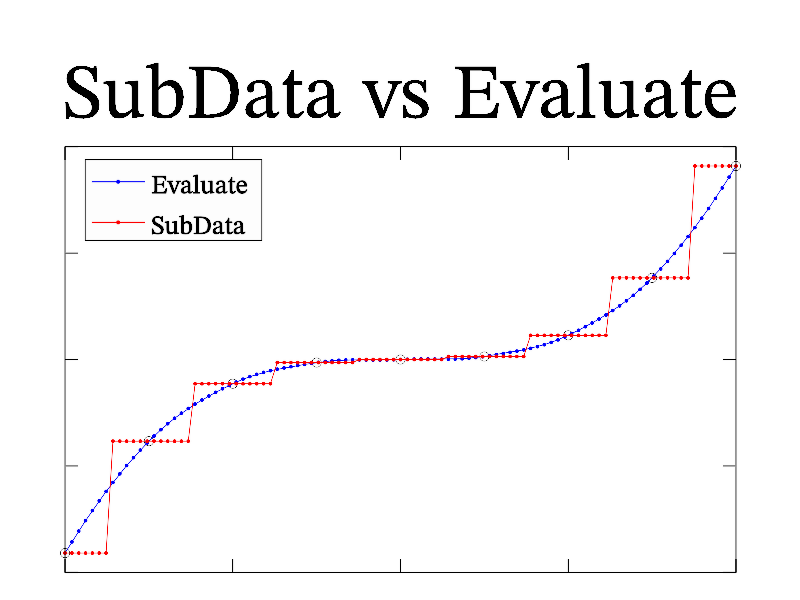
Example of datagrid usage is done in Making regular data. Here I want to show the peculiarities of refill and gspline functions. Both functions require argument(s) which provide coordinates of the data values, and return rectangular data array which equidistantly distributed in axis range. So, in opposite to evaluate function, refill and gspline can interpolate non-equidistantly distributed data. At this both functions refill and gspline provide continuity of 2nd derivatives along coordinate(s). However, refill is slower but give better (from human point of view) result than global spline gspline due to more advanced algorithm. Following sample illustrates this difference:
int sample(mglGraph *gr)
{
  mglData x(10), y(10), r(100);
  x.Modify("0.5+rnd");  x.CumSum("x");  x.Norm(-1,1);
  y.Modify("sin(pi*v)/1.5",x);
  gr->SubPlot(2,2,0,"<_");  gr->Title("Refill sample");
  gr->Axis();  gr->Box(); gr->Plot(x,y,"o ");
  gr->Refill(r,x,y);  // or you can use r.Refill(x,y,-1,1);
  gr->Plot(r,"r");  gr->FPlot("sin(pi*x)/1.5","B:");
  gr->SubPlot(2,2,1,"<_");gr->Title("Global spline");
  gr->Axis();  gr->Box(); gr->Plot(x,y,"o ");
  r.RefillGS(x,y,-1,1);   gr->Plot(r,"r");
  gr->FPlot("sin(pi*x)/1.5","B:");

  gr->Alpha(true);  gr->Light(true);
  mglData z(10,10), xx(10,10), yy(10,10), rr(100,100);
  y.Modify("0.5+rnd");  y.CumSum("x");  y.Norm(-1,1);
  for(int i=0;i<10;i++) for(int j=0;j<10;j++)
    z.a[i+10*j] = sin(M_PI*x.a[i]*y.a[j])/1.5;
  gr->SubPlot(2,2,2); gr->Title("2d regular");  gr->Rotate(40,60);
  gr->Axis();  gr->Box(); gr->Mesh(x,y,z,"k");
  gr->Refill(rr,x,y,z); gr->Surf(rr);

  gr->Fill(xx,"(x+1)/2*cos(y*pi/2-1)");
  gr->Fill(yy,"(x+1)/2*sin(y*pi/2-1)");
  for(int i=0;i<10*10;i++)
    z.a[i] = sin(M_PI*xx.a[i]*yy.a[i])/1.5;
  gr->SubPlot(2,2,3); gr->Title("2d non-regular");  gr->Rotate(40,60);
  gr->Axis();  gr->Box();  gr->Plot(xx,yy,z,"ko ");
  gr->Refill(rr,xx,yy,z);  gr->Surf(rr);
}
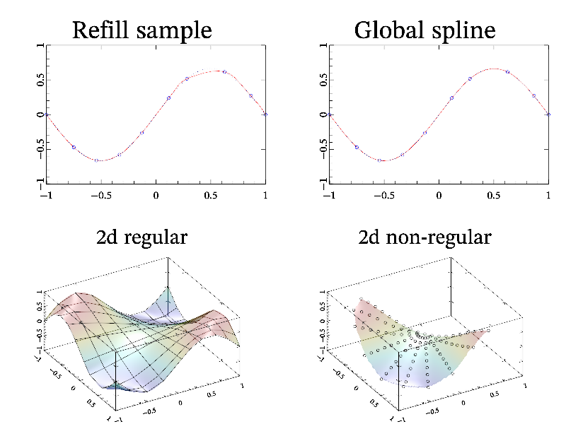
Next: Making histogram, Previous: Data interpolation, Up: Hints [Contents][Index]
Sometimes, one have only unregular data, like as data on triangular grids, or experimental results and so on. Such kind of data cannot be used as simple as regular data (like matrices). Only few functions, like dots, can handle unregular data as is.
However, one can use built in triangulation functions for interpolating unregular data points to a regular data grids. There are 2 ways. First way, one can use triangulation function to obtain list of vertexes for triangles. Later this list can be used in functions like triplot or tricont. Second way consist in usage of datagrid function, which fill regular data grid by interpolated values, assuming that coordinates of the data grid is equidistantly distributed in axis range. Note, you can use options (see Command options) to change default axis range as well as in other plotting functions.
int sample(mglGraph *gr)
{
  mglData x(100), y(100), z(100);
  gr->Fill(x,"2*rnd-1"); gr->Fill(y,"2*rnd-1"); gr->Fill(z,"v^2-w^2",x,y);
  // first way - plot triangular surface for points
  mglData d = mglTriangulation(x,y);
  gr->Title("Triangulation");
  gr->Rotate(40,60);	gr->Box();	gr->Light(true);
  gr->TriPlot(d,x,y,z);	gr->TriPlot(d,x,y,z,"#k");
  // second way - make regular data and plot it
  mglData g(30,30);
  gr->DataGrid(g,x,y,z);	gr->Mesh(g,"m");
}
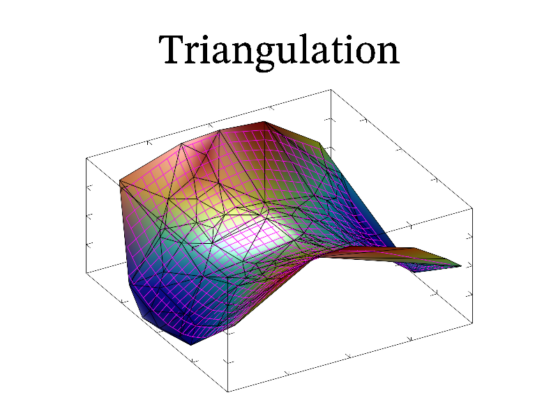
Next: Nonlinear fitting hints, Previous: Making regular data, Up: Hints [Contents][Index]
Using the hist function(s) for making regular distributions is one of useful fast methods to process and plot irregular data. Hist can be used to find some momentum of set of points by specifying weight function. It is possible to create not only 1D distributions but also 2D and 3D ones. Below I place the simplest sample code which demonstrate hist usage:
int sample(mglGraph *gr)
{
  mglData x(10000), y(10000), z(10000);  gr->Fill(x,"2*rnd-1");
  gr->Fill(y,"2*rnd-1"); gr->Fill(z,"exp(-6*(v^2+w^2))",x,y);
  mglData xx=gr->Hist(x,z), yy=gr->Hist(y,z);	xx.Norm(0,1);
  yy.Norm(0,1);
  gr->MultiPlot(3,3,3,2,2,"");   gr->SetRanges(-1,1,-1,1,0,1);
  gr->Box();  gr->Dots(x,y,z,"wyrRk");
  gr->MultiPlot(3,3,0,2,1,"");   gr->SetRanges(-1,1,0,1);
  gr->Box();  gr->Bars(xx);
  gr->MultiPlot(3,3,5,1,2,"");   gr->SetRanges(0,1,-1,1);
  gr->Box();  gr->Barh(yy);
  gr->SubPlot(3,3,2);
  gr->Puts(mglPoint(0.5,0.5),"Hist and\nMultiPlot\nsample","a",-6);
  return 0;
}
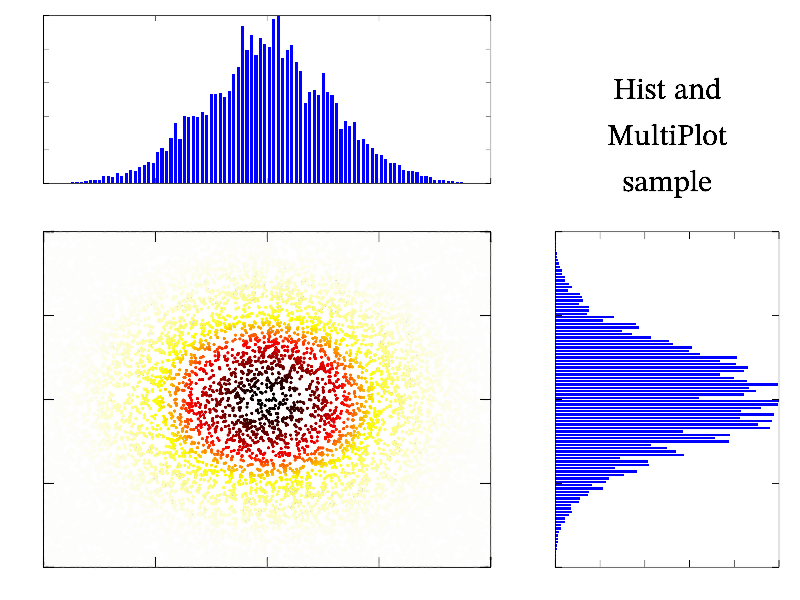
Next: PDE solving hints, Previous: Making histogram, Up: Hints [Contents][Index]
Nonlinear fitting is rather simple. All that you need is the data to fit, the approximation formula and the list of coefficients to fit (better with its initial guess values). Let me demonstrate it on the following simple example. First, let us use sin function with some random noise:
  mglData dat(100), in(100); //data to be fitted and ideal data
  gr->Fill(dat,"0.4*rnd+0.1+sin(2*pi*x)");
  gr->Fill(in,"0.3+sin(2*pi*x)");
and plot it to see that data we will fit
  gr->Title("Fitting sample");
  gr->SetRange('y',-2,2); gr->Box();  gr->Plot(dat, "k. ");
  gr->Axis(); gr->Plot(in, "b");
  gr->Puts(mglPoint(0, 2.2), "initial: y = 0.3+sin(2\\pi x)", "b");
The next step is the fitting itself. For that let me specify an initial values ini for coefficients ‘abc’ and do the fitting for approximation formula ‘a+b*sin(c*x)’
  mreal ini[3] = {1,1,3};
  mglData Ini(3,ini);
  mglData res = gr->Fit(dat, "a+b*sin(c*x)", "abc", Ini);
Now display it
  gr->Plot(res, "r");
  gr->Puts(mglPoint(-0.9, -1.3), "fitted:", "r:L");
  gr->PutsFit(mglPoint(0, -1.8), "y = ", "r");
NOTE! the fitting results may have strong dependence on initial values for coefficients due to algorithm features. The problem is that in general case there are several local "optimums" for coefficients and the program returns only first found one! There are no guaranties that it will be the best. Try for example to set ini[3] = {0, 0, 0} in the code above.
The full sample code for nonlinear fitting is:
int sample(mglGraph *gr)
{
  mglData dat(100), in(100);
  gr->Fill(dat,"0.4*rnd+0.1+sin(2*pi*x)");
  gr->Fill(in,"0.3+sin(2*pi*x)");
  mreal ini[3] = {1,1,3};
  mglData Ini(3,ini);

  mglData res = gr->Fit(dat, "a+b*sin(c*x)", "abc", Ini);

  gr->Title("Fitting sample");
  gr->SetRange('y',-2,2); gr->Box();  gr->Plot(dat, "k. ");
  gr->Axis();   gr->Plot(res, "r"); gr->Plot(in, "b");
  gr->Puts(mglPoint(-0.9, -1.3), "fitted:", "r:L");
  gr->PutsFit(mglPoint(0, -1.8), "y = ", "r");
  gr->Puts(mglPoint(0, 2.2), "initial: y = 0.3+sin(2\\pi x)", "b");
  return 0;
}
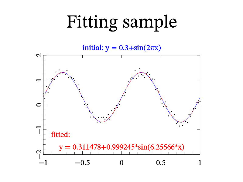
Next: Drawing phase plain, Previous: Nonlinear fitting hints, Up: Hints [Contents][Index]
Solving of Partial Differential Equations (PDE, including beam tracing) and ray tracing (or finding particle trajectory) are more or less common task. So, MathGL have several functions for that. There are ray for ray tracing, pde for PDE solving, qo2d for beam tracing in 2D case (see Global functions). Note, that these functions take “Hamiltonian” or equations as string values. And I don’t plan now to allow one to use user-defined functions. There are 2 reasons: the complexity of corresponding interface; and the basic nature of used methods which are good for samples but may not good for serious scientific calculations.
The ray tracing can be done by ray function. Really ray tracing equation is Hamiltonian equation for 3D space. So, the function can be also used for finding a particle trajectory (i.e. solve Hamiltonian ODE) for 1D, 2D or 3D cases. The function have a set of arguments. First of all, it is Hamiltonian which defined the media (or the equation) you are planning to use. The Hamiltonian is defined by string which may depend on coordinates ‘x’, ‘y’, ‘z’, time ‘t’ (for particle dynamics) and momentums ‘p’=p_x, ‘q’=p_y, ‘v’=p_z. Next, you have to define the initial conditions for coordinates and momentums at ‘t’=0 and set the integrations step (default is 0.1) and its duration (default is 10). The Runge-Kutta method of 4-th order is used for integration.
  const char *ham = "p^2+q^2-x-1+i*0.5*(y+x)*(y>-x)";
  mglData r = mglRay(ham, mglPoint(-0.7, -1), mglPoint(0, 0.5), 0.02, 2);
This example calculate the reflection from linear layer (media with Hamiltonian ‘p^2+q^2-x-1’=p_x^2+p_y^2-x-1). This is parabolic curve. The resulting array have 7 columns which contain data for {x,y,z,p,q,v,t}.
The solution of PDE is a bit more complicated. As previous you have to specify the equation as pseudo-differential operator \hat H(x, \nabla) which is called sometime as “Hamiltonian” (for example, in beam tracing). As previously, it is defined by string which may depend on coordinates ‘x’, ‘y’, ‘z’ (but not time!), momentums ‘p’=(d/dx)/i k_0, ‘q’=(d/dy)/i k_0 and field amplitude ‘u’=|u|. The evolutionary coordinate is ‘z’ in all cases. So that, the equation look like du/dz = ik_0 H(x,y,\hat p, \hat q, |u|)[u]. Dependence on field amplitude ‘u’=|u| allows one to solve nonlinear problems too. For example, for nonlinear Shrodinger equation you may set ham="p^2 + q^2 - u^2". Also you may specify imaginary part for wave absorption, like ham = "p^2 + i*x*(x>0)" or ham = "p^2 + i1*x*(x>0)".
Next step is specifying the initial conditions at ‘z’ equal to minimal z-axis value. The function need 2 arrays for real and for imaginary part. Note, that coordinates x,y,z are supposed to be in specified axis range. So, the data arrays should have corresponding scales. Finally, you may set the integration step and parameter k0=k_0. Also keep in mind, that internally the 2 times large box is used (for suppressing numerical reflection from boundaries) and the equation should well defined even in this extended range.
Final comment is concerning the possible form of pseudo-differential operator H. At this moment, simplified form of operator H is supported – all “mixed” terms (like ‘x*p’->x*d/dx) are excluded. For example, in 2D case this operator is effectively H = f(p,z) + g(x,z,u). However commutable combinations (like ‘x*q’->x*d/dy) are allowed for 3D case.
So, for example let solve the equation for beam deflected from linear layer and absorbed later. The operator will have the form ‘"p^2+q^2-x-1+i*0.5*(z+x)*(z>-x)"’ that correspond to equation 1/ik_0 * du/dz + d^2 u/dx^2 + d^2 u/dy^2 + x * u + i (x+z)/2 * u = 0. This is typical equation for Electron Cyclotron (EC) absorption in magnetized plasmas. For initial conditions let me select the beam with plane phase front exp(-48*(x+0.7)^2). The corresponding code looks like this:
int sample(mglGraph *gr)
{
  mglData a,re(128),im(128);
  gr->Fill(re,"exp(-48*(x+0.7)^2)");
  a = gr->PDE("p^2+q^2-x-1+i*0.5*(z+x)*(z>-x)", re, im, 0.01, 30);
  a.Transpose("yxz");
  gr->SubPlot(1,1,0,"<_"); gr->Title("PDE solver");
  gr->SetRange('c',0,1);  gr->Dens(a,"wyrRk");
  gr->Axis(); gr->Label('x', "\\i x");  gr->Label('y', "\\i z");
  gr->FPlot("-x", "k|");
  gr->Puts(mglPoint(0, 0.85), "absorption: (x+z)/2 for x+z>0");
  gr->Puts(mglPoint(0,1.1),"Equation: ik_0\\partial_zu + \\Delta u + x\\cdot u + i \\frac{x+z}{2}\\cdot u = 0");
  return 0;
}
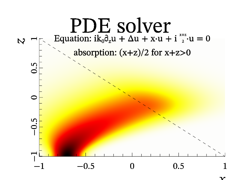
The next example is the beam tracing. Beam tracing equation is special kind of PDE equation written in coordinates accompanied to a ray. Generally this is the same parameters and limitation as for PDE solving but the coordinates are defined by the ray and by parameter of grid width w in direction transverse the ray. So, you don’t need to specify the range of coordinates. BUT there is limitation. The accompanied coordinates are well defined only for smooth enough rays, i.e. then the ray curvature K (which is defined as 1/K^2 = (|r''|^2 |r'|^2 - (r'', r'')^2)/|r'|^6) is much large then the grid width: K>>w. So, you may receive incorrect results if this condition will be broken.
You may use following code for obtaining the same solution as in previous example:
int sample(mglGraph *gr)
{
  mglData r, xx, yy, a, im(128), re(128);
  const char *ham = "p^2+q^2-x-1+i*0.5*(y+x)*(y>-x)";
  r = mglRay(ham, mglPoint(-0.7, -1), mglPoint(0, 0.5), 0.02, 2);
  gr->SubPlot(1,1,0,"<_"); gr->Title("Beam and ray tracing");
  gr->Plot(r.SubData(0), r.SubData(1), "k");
  gr->Axis(); gr->Label('x', "\\i x");  gr->Label('y', "\\i z");

  // now start beam tracing
  gr->Fill(re,"exp(-48*x^2)");
  a = mglQO2d(ham, re, im, r, xx, yy, 1, 30);
  gr->SetRange('c',0, 1);
  gr->Dens(xx, yy, a, "wyrRk");
  gr->FPlot("-x", "k|");
  gr->Puts(mglPoint(0, 0.85), "absorption: (x+y)/2 for x+y>0");
  gr->Puts(mglPoint(0.7, -0.05), "central ray");
  return 0;
}
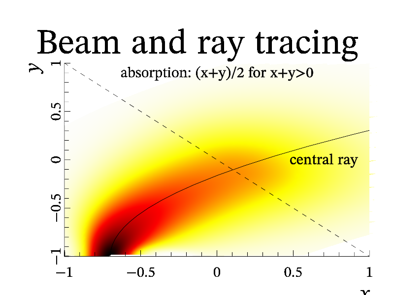
Note, the pde is fast enough and suitable for many cases routine. However, there is situations then media have both together: strong spatial dispersion and spatial inhomogeneity. In this, case the pde will produce incorrect result and you need to use advanced PDE solver apde. For example, a wave beam, propagated in plasma, described by Hamiltonian exp(-x^2-p^2), will have different solution for using of simplification and advanced PDE solver:
int sample(mglGraph *gr)
{
  gr->SetRanges(-1,1,0,2,0,2);
  mglData ar(256), ai(256);	gr->Fill(ar,"exp(-2*x^2)");

  mglData res1(gr->APDE("exp(-x^2-p^2)",ar,ai,0.01));	res1.Transpose();
  gr->SubPlot(1,2,0,"_");	gr->Title("Advanced PDE solver");
  gr->SetRanges(0,2,-1,1);	gr->SetRange('c',res1);
  gr->Dens(res1);	gr->Axis();	gr->Box();
  gr->Label('x',"\\i z");	gr->Label('y',"\\i x");
  gr->Puts(mglPoint(-0.5,0.2),"i\\partial_z\\i u = exp(-\\i x^2+\\partial_x^2)[\\i u]","y");

  mglData res2(gr->PDE("exp(-x^2-p^2)",ar,ai,0.01));
  gr->SubPlot(1,2,1,"_");	gr->Title("Simplified PDE solver");
  gr->Dens(res2);	gr->Axis();	gr->Box();
  gr->Label('x',"\\i z");	gr->Label('y',"\\i x");
  gr->Puts(mglPoint(-0.5,0.2),"i\\partial_z\\i u \\approx\\ exp(-\\i x^2)\\i u+exp(\\partial_x^2)[\\i u]","y");
  return 0;
}
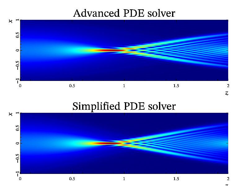
Next: Pulse properties, Previous: PDE solving hints, Up: Hints [Contents][Index]
Here I want say a few words of plotting phase plains. Phase plain is name for system of coordinates x, x', i.e. a variable and its time derivative. Plot in phase plain is very useful for qualitative analysis of an ODE, because such plot is rude (it topologically the same for a range of ODE parameters). Most often the phase plain {x, x'} is used (due to its simplicity), that allows to analyze up to the 2nd order ODE (i.e. x''+f(x,x')=0).
The simplest way to draw phase plain in MathGL is using flow function(s), which automatically select several points and draw flow threads. If the ODE have an integral of motion (like Hamiltonian H(x,x')=const for dissipation-free case) then you can use cont function for plotting isolines (contours). In fact. isolines are the same as flow threads, but without arrows on it. Finally, you can directly solve ODE using ode function and plot its numerical solution.
Let demonstrate this for ODE equation x''-x+3*x^2=0. This is nonlinear oscillator with square nonlinearity. It has integral H=y^2+2*x^3-x^2=Const. Also it have 2 typical stationary points: saddle at {x=0, y=0} and center at {x=1/3, y=0}. Motion at vicinity of center is just simple oscillations, and is stable to small variation of parameters. In opposite, motion around saddle point is non-stable to small variation of parameters, and is very slow. So, calculation around saddle points are more difficult, but more important. Saddle points are responsible for solitons, stochasticity and so on.
So, let draw this phase plain by 3 different methods. First, draw isolines for H=y^2+2*x^3-x^2=Const – this is simplest for ODE without dissipation. Next, draw flow threads – this is straightforward way, but the automatic choice of starting points is not always optimal. Finally, use ode to check the above plots. At this we need to run ode in both direction of time (in future and in the past) to draw whole plain. Alternatively, one can put starting points far from (or at the bounding box as done in flow) the plot, but this is a more complicated. The sample code is:
int sample(mglGraph *gr)
{
  gr->SubPlot(2,2,0,"<_");  gr->Title("Cont");  gr->Box();
  gr->Axis();  gr->Label('x',"x");  gr->Label('y',"\\dot{x}");
  mglData f(100,100);   gr->Fill(f,"y^2+2*x^3-x^2-0.5");
  gr->Cont(f);
  gr->SubPlot(2,2,1,"<_");  gr->Title("Flow");  gr->Box();
  gr->Axis();  gr->Label('x',"x");  gr->Label('y',"\\dot{x}");
  mglData fx(100,100), fy(100,100);
  gr->Fill(fx,"x-3*x^2");  gr->Fill(fy,"y");
  gr->Flow(fy,fx,"v","value 7");
  gr->SubPlot(2,2,2,"<_");  gr->Title("ODE");   gr->Box();
  gr->Axis();  gr->Label('x',"x");  gr->Label('y',"\\dot{x}");
  for(double x=-1;x<1;x+=0.1)
  {
    mglData in(2), r;   in.a[0]=x;
    r = mglODE("y;x-3*x^2","xy",in);
    gr->Plot(r.SubData(0), r.SubData(1));
    r = mglODE("-y;-x+3*x^2","xy",in);
    gr->Plot(r.SubData(0), r.SubData(1));
  }
}
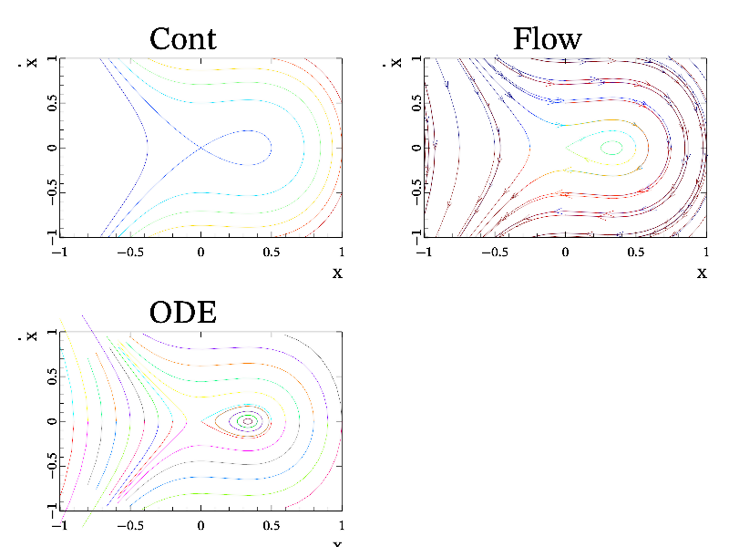
Next: Using MGL parser, Previous: Drawing phase plain, Up: Hints [Contents][Index]
There is common task in optics to determine properties of wave pulses or wave beams. MathGL provide special function pulse which return the pulse properties (maximal value, center of mass, width and so on). Its usage is rather simple. Here I just illustrate it on the example of Gaussian pulse, where all parameters are obvious.
void sample(mglGraph *gr)
{
  gr->SubPlot(1,1,0,"<_");  gr->Title("Pulse sample");
  // first prepare pulse itself
  mglData a(100); gr->Fill(a,"exp(-6*x^2)");
  // get pulse parameters
  mglData b(a.Pulse('x'));
  // positions and widths are normalized on the number of points. So, set proper axis scale.
  gr->SetRanges(0, a.nx-1, 0, 1);
  gr->Axis(); gr->Plot(a);  // draw pulse and axis
  // now visualize found pulse properties
  double m = b[0];  // maximal amplitude
  // approximate position of maximum
  gr->Line(mglPoint(b[1],0), mglPoint(b[1],m),"r=");
  // width at half-maximum (so called FWHM)
  gr->Line(mglPoint(b[1]-b[3]/2,0), mglPoint(b[1]-b[3]/2,m),"m|");
  gr->Line(mglPoint(b[1]+b[3]/2,0), mglPoint(b[1]+b[3]/2,m),"m|");
  gr->Line(mglPoint(0,m/2), mglPoint(a.nx-1,m/2),"h");
  // parabolic approximation near maximum
  char func[128];	sprintf(func,"%g*(1-((x-%g)/%g)^2)",b[0],b[1],b[2]);
  gr->FPlot(func,"g");
}
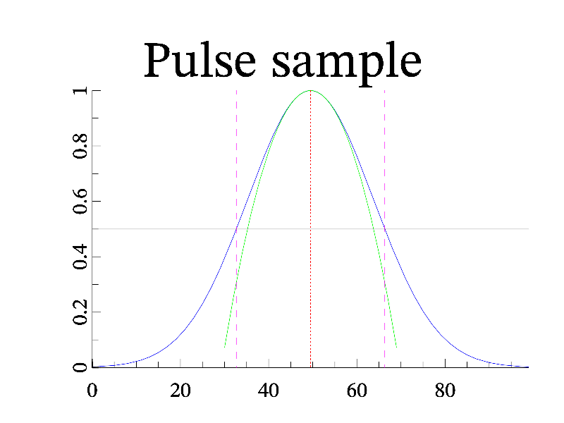
Next: Using options, Previous: Pulse properties, Up: Hints [Contents][Index]
Sometimes you may prefer to use MGL scripts in yours code. It is simpler (especially in comparison with C/Fortran interfaces) and provide faster way to plot the data with annotations, labels and so on. Class mglParse (see mglParse class parse MGL scripts in C++. It have also the corresponding interface for C/Fortran.
The key function here is mglParse::Parse() (or mgl_parse() for C/Fortran) which execute one command per string. At this the detailed information about the possible errors or warnings is passed as function value. Or you may execute the whole script as long string with lines separated by ‘\n’. Functions mglParse::Execute() and mgl_parse_text() perform it. Also you may set the values of parameters ‘$0’...‘$9’ for the script by functions mglParse::AddParam() or mgl_add_param(), allow/disable picture resizing, check “once” status and so on. The usage is rather straight-forward.
The only non-obvious thing is data transition between script and yours program. There are 2 stages: add or find variable; and set data to variable. In C++ you may use functions mglParse::AddVar() and mglParse::FindVar() which return pointer to mglData. In C/Fortran the corresponding functions are mgl_add_var(), mgl_find_var(). This data pointer is valid until next Parse() or Execute() call. Note, you must not delete or free the data obtained from these functions!
So, some simple example at the end. Here I define a data array, create variable, put data into it and plot it. The C++ code looks like this:
int sample(mglGraph *gr)
{
  gr->Title("MGL parser sample");
  mreal a[100];   // let a_i = sin(4*pi*x), x=0...1
  for(int i=0;i<100;i++)a[i]=sin(4*M_PI*i/99);
  mglParse *parser = new mglParse;
  mglData *d = parser->AddVar("dat");
  d->Set(a,100); // set data to variable
  parser->Execute(gr, "plot dat; xrange 0 1\nbox\naxis");
  // you may break script at any line do something
  // and continue after that
  parser->Execute(gr, "xlabel 'x'\nylabel 'y'\nbox");
  // also you may use cycles or conditions in script
  parser->Execute(gr, "for $0 -1 1 0.1\nif $0<0\n"
    "line 0 0 -1 $0 'r':else:line 0 0 -1 $0 'g'\n"
    "endif\nnext");
  delete parser;
  return 0;
}
The code in C/Fortran looks practically the same:
int sample(HMGL gr)
{
  mgl_title(gr, "MGL parser sample", "", -2);
  double a[100];   // let a_i = sin(4*pi*x), x=0...1
  int i;
  for(i=0;i<100;i++)  a[i]=sin(4*M_PI*i/99);
  HMPR parser = mgl_create_parser();
  HMDT d = mgl_parser_add_var(parser, "dat");
  mgl_data_set_double(d,a,100,1,1);    // set data to variable
  mgl_parse_text(gr, parser, "plot dat; xrange 0 1\nbox\naxis");
  // you may break script at any line do something
  // and continue after that
  mgl_parse_text(gr, parser, "xlabel 'x'\nylabel 'y'");
  // also you may use cycles or conditions in script
  mgl_parse_text(gr, parser, "for $0 -1 1 0.1\nif $0<0\n"
    "line 0 0 -1 $0 'r':else:line 0 0 -1 $0 'g'\n"
    "endif\nnext");
  mgl_write_png(gr, "test.png", "");  // don't forgot to save picture
  return 0;
}

Next: ``Templates'', Previous: Using MGL parser, Up: Hints [Contents][Index]
Command options allow the easy setup of the selected plot by changing global settings only for this plot. Often, options are used for specifying the range of automatic variables (coordinates). However, options allows easily change plot transparency, numbers of line or faces to be drawn, or add legend entries. The sample function for options usage is:
void template(mglGraph *gr)
{
  mglData a(31,41);
  gr->Fill(a,"-pi*x*exp(-(y+1)^2-4*x^2)");

  gr->SubPlot(2,2,0);	gr->Title("Options for coordinates");
  gr->Alpha(true);	gr->Light(true);
  gr->Rotate(40,60);    gr->Box();
  gr->Surf(a,"r","yrange 0 1"); gr->Surf(a,"b","yrange 0 -1");
  if(mini)	return;
  gr->SubPlot(2,2,1);   gr->Title("Option 'meshnum'");
  gr->Rotate(40,60);    gr->Box();
  gr->Mesh(a,"r","yrange 0 1"); gr->Mesh(a,"b","yrange 0 -1; meshnum 5");
  gr->SubPlot(2,2,2);   gr->Title("Option 'alpha'");
  gr->Rotate(40,60);    gr->Box();
  gr->Surf(a,"r","yrange 0 1; alpha 0.7");
  gr->Surf(a,"b","yrange 0 -1; alpha 0.3");
  gr->SubPlot(2,2,3,"<_");  gr->Title("Option 'legend'");
  gr->FPlot("x^3","r","legend 'y = x^3'");
  gr->FPlot("cos(pi*x)","b","legend 'y = cos \\pi x'");
  gr->Box();    gr->Axis(); gr->Legend(2,"");
}

Next: Stereo image, Previous: Using options, Up: Hints [Contents][Index]
As I have noted before, the change of settings will influence only for the further plotting commands. This allows one to create “template” function which will contain settings and primitive drawing for often used plots. Correspondingly one may call this template-function for drawing simplification.
For example, let one has a set of points (experimental or numerical) and wants to compare it with theoretical law (for example, with exponent law \exp(-x/2), x \in [0, 20]). The template-function for this task is:
void template(mglGraph *gr)
{
  mglData  law(100);      // create the law
  law.Modify("exp(-10*x)");
  gr->SetRanges(0,20, 0.0001,1);
  gr->SetFunc(0,"lg(y)",0);
  gr->Plot(law,"r2");
  gr->Puts(mglPoint(10,0.2),"Theoretical law: e^x","r:L");
  gr->Label('x',"x val."); gr->Label('y',"y val.");
  gr->Axis(); gr->Grid("xy","g;"); gr->Box();
}
At this, one will only write a few lines for data drawing:
  template(gr);     // apply settings and default drawing from template
  mglData dat("fname.dat"); // load the data
  // and draw it (suppose that data file have 2 columns)
  gr->Plot(dat.SubData(0),dat.SubData(1),"bx ");
A template-function can also contain settings for font, transparency, lightning, color scheme and so on.
I understand that this is obvious thing for any professional programmer, but I several times receive suggestion about “templates” ... So, I decide to point out it here.
Next: Reduce memory usage, Previous: ``Templates'', Up: Hints [Contents][Index]
One can easily create stereo image in MathGL. Stereo image can be produced by making two subplots with slightly different rotation angles. The corresponding code looks like this:
int sample(mglGraph *gr)
{
  mglData a;  mgls_prepare2d(&a);
  gr->Light(true);

  gr->SubPlot(2,1,0); gr->Rotate(50,60+1);
  gr->Box();  gr->Surf(a);

  gr->SubPlot(2,1,1); gr->Rotate(50,60-1);
  gr->Box();  gr->Surf(a);
  return 0;
}

Next: Saving and scanning file, Previous: Stereo image, Up: Hints [Contents][Index]
By default MathGL save all primitives in memory, rearrange it and only later draw them on bitmaps. Usually, this speed up drawing, but may require a lot of memory for plots which contain a lot of faces (like cloud, dew). You can use quality function for setting to use direct drawing on bitmap and bypassing keeping any primitives in memory. This function also allow you to decrease the quality of the resulting image but increase the speed of the drawing.
The code for lowest memory usage looks like this:
int sample(mglGraph *gr)
{
  gr->SetQuality(6);   // firstly, set to draw directly on bitmap
  for(i=0;i<1000;i++)
    gr->Sphere(mglPoint(mgl_rnd()*2-1,mgl_rnd()*2-1),0.05);
  return 0;
}
Next: Mixing bitmap and vector output, Previous: Reduce memory usage, Up: Hints [Contents][Index]
MathGL have possibilities to write textual information into file with variable values. In MGL script you can use save command for that. However, the usual printf(); is simple in C/C++ code. For example, lets create some textual file
FILE *fp=fopen("test.txt","w");
fprintf(fp,"This is test: 0 -> 1 q\n");
fprintf(fp,"This is test: 1 -> -1 q\n");
fprintf(fp,"This is test: 2 -> 0 q\n");
fclose(fp);
It contents look like
This is test: 0 -> 1 q
This is test: 1 -> -1 q
This is test: 2 -> 0 q
Let assume now that you want to read this values (i.e. [[0,1],[1,-1],[2,0]]) from the file. You can use scanfile for that. The desired values was written using template "This is test: %g -> %g q\n". So, just use
mglData a;
a.ScanFile("test.txt","This is test: %g -> %g");
and plot it to for assurance
gr->SetRanges(a.SubData(0), a.SubData(1));
gr->Axis();	gr->Plot(a.SubData(0),a.SubData(1),"o");
Note, I keep only the leading part of template (i.e. "This is test: %g -> %g" instead of "This is test: %g -> %g q\n"), because there is no important for us information after the second number in the line.
Previous: Saving and scanning file, Up: Hints [Contents][Index]
Sometimes output plots contain surfaces with a lot of points, and some vector primitives (like axis, text, curves, etc.). Using vector output formats (like EPS or SVG) will produce huge files with possible loss of smoothed lighting. Contrary, the bitmap output may cause the roughness of text and curves. Hopefully, MathGL have a possibility to combine bitmap output for surfaces and vector one for other primitives in the same EPS file, by using rasterize command.
The idea is to prepare part of picture with surfaces or other "heavy" plots and produce the background image from them by help of rasterize command. Next, we draw everything to be saved in vector form (text, curves, axis and etc.). Note, that you need to clear primitives (use clf command) after rasterize if you want to disable duplication of surfaces in output files (like EPS). Note, that some of output formats (like 3D ones, and TeX) don’t support the background bitmap, and use clf for them will cause the loss of part of picture.
The sample code is:
// first draw everything to be in bitmap output
gr->FSurf("x^2+y^2", "#", "value 10");

gr->Rasterize();  // set above plots as bitmap background
gr->Clf();        // clear primitives, to exclude them from file

// now draw everything to be in vector output
gr->Axis(); gr->Box();

// and save file
gr->WriteFrame("fname.eps");
Check that points of the plot are located inside the bounding box and resize the bounding box using ranges function. Check that the data have correct dimensions for selected type of plot. Be sure that Finish() is called after the plotting functions (or be sure that the plot is saved to a file). Sometimes the light reflection from flat surfaces (like, dens) can look as if the plot were absent.
Most “new” types of plots can be created by using the existing drawing functions. For example, the surface of curve rotation can be created by a special function torus, or as a parametrically specified surface by surf. See also, Hints. If you can not find a specific type of plot, please e-mail me and this plot will appear in the next version of MathGL library.
No. The MathGL library is self-contained and does not require the knowledge of external libraries.
The core of the MathGL library is written in C++. But there are interfaces for: pure C, Fortran, Pascal, Forth, and its own command language MGL. Also there is a large set of interpreted languages, which are supported (Python, Java, ALLEGROCL, CHICKEN, Lisp, CFFI, C#, Guile, Lua, Modula 3, Mzscheme, Ocaml, Octave, Perl, PHP, Pike, R, Ruby, Tcl). These interfaces are written using SWIG (both pure C functions and classes) but only the interface for Python and Octave is included in the build system. The reason is that I don’t know any other interpreted languages :(. Note that most other languages can use (link to) the pure C functions.
You can use MathGL as is with gfortran because it uses by default the AT&T notation for external functions. For other compilers (like Visual Fortran) you have to switch on the AT&T notation manually. The AT&T notation requires that the symbol ‘_’ is added at the end of each function name, function argument(s) is passed by pointers and the string length(s) is passed at the end of the argument list. For example:
C function – void mgl_fplot(HMGL graph, const char *fy, const char *stl, int n);
AT&T function – void mgl_fplot_(uintptr_t *graph, const char *fy, const char *stl, int *n, int ly, int ls);
Fortran users also should add C++ library by the option -lstdc++. If library was built with enable-double=ON (this default for v.2.1 and later) then all real numbers must be real*8. You can make it automatic if use option -fdefault-real-8.
The standard way is to use Unicode encoding for the text output. But the MathGL library also has interface for 8-bit (char *) strings with internal conversion to Unicode. This conversion depends on the current locale OS. You may change it by setlocale() function. For example, for Russian text in CP1251 encoding you may use setlocale(LC_CTYPE, "ru_RU.cp1251"); (under MS Windows the name of locale may differ – setlocale(LC_CTYPE, "russian_russia.1251")). I strongly recommend not to use the constant LC_ALL in the conversion. Since it also changes the number format, it may lead to mistakes in formula writing and reading of the text in data files. For example, the program will await a ‘,’ as a decimal point but the user will enter ‘.’.
There are 3 general ways. First, the point with NAN value as one of the coordinates (including color/alpha range) will never be plotted. Second, special functions SetCutBox() and CutOff() define the condition when the points should be omitted (see Cutting). Last, you may change the transparency of a part of the plot by the help of functions surfa, surf3a (see Dual plotting). In last case the transparency is switched on smoothly.
In version 2.0, main classes (mglGraph and mglData) contains only inline functions and are acceptable for any compiler with the same binary files. However, if you plan to use widget classes (QMathGL, Fl_MathGL, ...) or to access low-level features (mglBase, mglCanvas, ...) then you have to recompile MathGL by yours compiler.
Note, that you have to make import library(-ies) *.lib for provided binary *.dll. This procedure depend on used compiler – please read documentation for yours compiler. For VisualStudio, it can be done by command lib.exe /DEF:libmgl.def /OUT:libmgl.lib.
You need to put yours calculations or main event-handling loop in the separate thread. For static image you can give NULL as drawing function and call Update() function when you need to redraw it. For more details see Animation.
Generally, it is the same procedure as for Linux or MacOS – see section Installation. The simplest way is using the combination CMake+MinGW. Also you may need some extra libraries like GSL, PNG, JPEG and so on. All of them can be found at http://gnuwin32.sourceforge.net/packages.html. After installing all components, just run cmake-gui configurator and build the MathGL itself.
Most of the library was written by one person. This is a result of nearly a year of work (mostly in the evening and on holidays): I spent half a year to write the kernel and half a year to a year on extending, improving the library and writing documentation. This process continues now :). The build system (cmake files) was written mostly by D.Kulagin, and the export to PRC/PDF was written mostly by M.Vidassov.
You can import data into a mglData instance by function import and display it by dens function. For example, for black-and-white bitmap you can use the code: mglData bmp; bmp.Import("fname.png","wk"); gr->Dens(bmp,"wk");.
There are special classes (widgets) for these libraries: QMathGL for Qt, Fl_MathGL for FLTK and so on. If you don’t find the appropriate class then you can create your own widget that displays a bitmap using mglCanvas::GetRGB().
Just use WritePRC() method which also create PDF file if enable-pdf=ON at MathGL configure.
Just use WriteTEX() method which create LaTeX files with figure itself ‘fname.tex’, with MathGL colors ‘mglcolors.tex’ and main file ‘mglmain.tex’. Last one can be used for viewing image by command like pdflatex mglmain.tex.
Yes, sample JavaScript file is located in texinfo/ folder of sources. You should provide JSON data with 3d image for it (can be created by WriteJSON() method). Script allows basic manipulation with plot: zoom, rotation, shift. Sample of JavaScript pictures can be found in http://mathgl.sf.net/json.html.
First, you should download new font files from here or from here. Next, you should load the font files into mglGraph class instance gr by the following command: gr->LoadFont(fontname,path);. Here fontname is the base font name like ‘STIX’ and path sets the location of font files. Use gr->RestoreFont(); to start using the default font.
Just set a negative value in ticklen. For example, use gr->SetTickLen(-0.1);.
Just use SetRotatedText(false). Also you can use axis style ‘U’ for disable only tick labels rotation.
*.so? What is gcc? How I can use make?They are standard GNU tools. There is special FAQ about its usage under Windows – http://www.mingw.org/wiki/FAQ.
Just use Aspect(NAN,NAN) for each subplot, or at the beginning of the drawing.
Just use code like Clf("r{A5}"); or prepare PNG file and set it as background image by call LoadBackground("fname.png");.
The simplest way is to use subplot style. However, you should be careful if you plan to add colorbar or rotate plot – part of plot can be invisible if you will use non-default subplot style.
Yes. Sometimes you may have huge surface and a small set of curves and/or text on the plot. You can use function rasterize just after making surface plot. This will put all plot to bitmap background. At this later plotting will be in vector format. For example, you can do something like following:
gr->Surf(x, y, z);
gr->Rasterize(); // make surface as bitmap
gr->Axis();
gr->WriteFrame("fname.eps");
MathGL support C99 standard, where ‘I’ is reserved for imaginary unit. If you still need this name, then just use
#undef I
after including MathGL header files.
You can save each frame into JPEG with names like ‘frame0001.jpg’, ‘frame0002.jpg’, ... Later you can use ImageMagic to convert them into MPEG video by command convert frame*.jpg movie.mpg. See also MPEG.
Next: MathGL core, Previous: Examples, Up: Top [Contents][Index]
The set of MathGL features is rather rich – just the number of basic graphics types is larger than 50. Also there are functions for data handling, plot setup and so on. In spite of it I tried to keep a similar style in function names and in the order of arguments. Mostly it is used for different drawing functions.
There are six most general (base) concepts:
SetQuality(MGL_DRAW_LMEM) or quality 6) or the list of vector primitives (default). After that the user may decide what he/she want: save to file, display on the screen, run animation, do additional editing and so on. This approach assures a high portability of the program – the source code will produce exactly the same picture in any OS. Another big positive consequence is the ability to create the picture in the console program (using command line, without creating a window)!
In addition to the general concepts I want to comment on some non-trivial or less commonly used general ideas – plot positioning, axis specification and curvilinear coordinates, styles for lines, text and color scheme.
| • Coordinate axes | ||
| • Color styles | ||
| • Line styles | ||
| • Color scheme | ||
| • Font styles | ||
| • Textual formulas | ||
| • Command options | ||
| • Interfaces |
Next: Color styles, Up: General concepts [Contents][Index]
Two axis representations are used in MathGL. The first one consists of normalizing coordinates of data points in axis range (see Axis settings). If SetCut() is true then the outlier points are omitted, otherwise they are projected to the bounding box (see Cutting). Also, the point will be omitted if it lies inside the box defined by SetCutBox() or if the value of formula CutOff() is nonzero for its coordinates. After that, transformation formulas defined by SetFunc() or SetCoor() are applied to the data point (see Curved coordinates). Finally, the data point is plotted by one of the functions.
The range of x, y, z-axis can be specified by SetRange() or ranges functions. Its origin is specified by origin function. At this you can you can use NAN values for selecting axis origin automatically.
There is 4-th axis c (color axis or colorbar) in addition to the usual axes x, y, z. It sets the range of values for the surface coloring. Its borders are automatically set to values of z-range during the call of ranges function. Also, one can directly set it by call SetRange('c', ...). Use colorbar function for drawing the colorbar.
The form (appearence) of tick labels is controlled by SetTicks() function (see Ticks). Function SetTuneTicks switches on/off tick enhancing by factoring out acommon multiplier (for small coordinate values, like 0.001 to 0.002, or large, like from 1000 to 2000) or common component (for narrow range, like from 0.999 to 1.000). Finally, you may use functions SetTickTempl() for setting templates for tick labels (it supports TeX symbols). Also, there is a possibility to print arbitrary text as tick labels the by help of SetTicksVal() function.
Next: Line styles, Previous: Coordinate axes, Up: General concepts [Contents][Index]
Base colors are defined by one of symbol ‘wkrgbcymhRGBCYMHWlenupqLENUPQ’.
The color types are: ‘k’ – black, ‘r’ – red, ‘R’ – dark red, ‘g’ – green, ‘G’ – dark green, ‘b’ – blue, ‘B’ – dark blue, ‘c’ – cyan, ‘C’ – dark cyan, ‘m’ – magenta, ‘M’ – dark magenta, ‘y’ – yellow, ‘Y’ – dark yellow (gold), ‘h’ – gray, ‘H’ – dark gray, ‘w’ – white, ‘W’ – bright gray, ‘l’ – green-blue, ‘L’ – dark green-blue, ‘e’ – green-yellow, ‘E’ – dark green-yellow, ‘n’ – sky-blue, ‘N’ – dark sky-blue, ‘u’ – blue-violet, ‘U’ – dark blue-violet, ‘p’ – purple, ‘P’ – dark purple, ‘q’ – orange, ‘Q’ – dark orange (brown).
You can also use “bright” colors. The “bright” color contain 2 symbols in brackets ‘{cN}’: first one is the usual symbol for color id, the second one is a digit for its brightness. The digit can be in range ‘1’...‘9’. Number ‘5’ corresponds to a normal color, ‘1’ is a very dark version of the color (practically black), and ‘9’ is a very bright version of the color (practically white). For example, the colors can be ‘{b2}’ ‘{b7}’ ‘{r7}’ and so on.
Finally, you can specify RGB or RGBA values of a color using format ‘{xRRGGBB}’ or ‘{xRRGGBBAA}’ correspondingly. For example, ‘{xFF9966}’ give you melone color.
Next: Color scheme, Previous: Color styles, Up: General concepts [Contents][Index]
The line style is defined by the string which may contain specifications for color (‘wkrgbcymhRGBCYMHWlenupqLENUPQ’), dashing style (‘-|;:ji=’ or space), width (‘123456789’) and marks (‘*o+xsd.^v<>’ and ‘#’ modifier). If one of the type of information is omitted then default values used with next color from palette (see Palette and colors). Note, that internal color counter will be nullified by any change of palette. This includes even hidden change (for example, by box or axis functions). By default palette contain following colors: dark gray ‘H’, blue ‘b’, green ‘g’, red ‘r’, cyan ‘c’, magenta ‘m’, yellow ‘y’, gray ‘h’, green-blue ‘l’, sky-blue ‘n’, orange ‘q’, green-yellow ‘e’, blue-violet ‘u’, purple ‘p’.
Dashing style has the following meaning: space – no line (usable for plotting only marks), ‘-’ – solid line (■■■■■■■■■■■■■■■■), ‘|’ – long dashed line (■■■■■■■■□□□□□□□□), ‘;’ – dashed line (■■■■□□□□■■■■□□□□), ‘=’ – small dashed line (■■□□■■□□■■□□■■□□), ‘:’ – dotted line (■□□□■□□□■□□□■□□□), ‘j’ – dash-dotted line (■■■■■■■□□□□■□□□□), ‘i’ – small dash-dotted line (■■■□□■□□■■■□□■□□), ‘{dNNNN}’ – manual dash style (for v.2.3 and later, like ‘{df090}’ for (■■■■□□□□■□□■□□□□)).
Marker types are: ‘o’ – circle, ‘+’ – cross, ‘x’ – skew cross, ‘s’ – square, ‘d’ – rhomb (or diamond), ‘.’ – dot (point), ‘^’ – triangle up, ‘v’ – triangle down, ‘<’ – triangle left, ‘>’ – triangle right, ‘#*’ – Y sign, ‘#+’ – squared cross, ‘#x’ – squared skew cross, ‘#.’ – circled dot. If string contain symbol ‘#’ then the solid versions of markers are used.
You can provide user-defined symbols (see addsymbol) to draw it as marker by using ‘&’ style. In particular, ‘&*’, ‘&o’, ‘&+’, ‘&x’, ‘&s’, ‘&d’, ‘&.’, ‘&^’, ‘&v’, ‘&<’, ‘&>’ will draw user-defined symbol ‘*o+xsd.^v<>’ correspondingly; and
‘&#o’, ‘&#+’, ‘&#x’, ‘&#s’, ‘&#d’, ‘&#.’, ‘&#^’, ‘&#v’, ‘&#<’, ‘&#>’ will draw user-defined symbols ‘YOPXSDCTVLR’ correspondingly. Note, that wired version of user-defined symbols will be drawn if you set negative marker size (see marksize or size in Command options).
One may specify to draw a special symbol (an arrow) at the beginning and at the end of line. This is done if the specification string contains one of the following symbols: ‘A’ – outer arrow, ‘V’ – inner arrow, ‘I’ – transverse hatches, ‘K’ – arrow with hatches, ‘T’ – triangle, ‘S’ – square, ‘D’ – rhombus, ‘O’ – circle, ‘X’ – skew cross, ‘_’ – nothing (the default). The following rule applies: the first symbol specifies the arrow at the end of line, the second specifies the arrow at the beginning of the line. For example, ‘r-A’ defines a red solid line with usual arrow at the end, ‘b|AI’ defines a blue dash line with an arrow at the end and with hatches at the beginning, ‘_O’ defines a line with the current style and with a circle at the beginning. These styles are applicable during the graphics plotting as well (for example, 1D plotting).
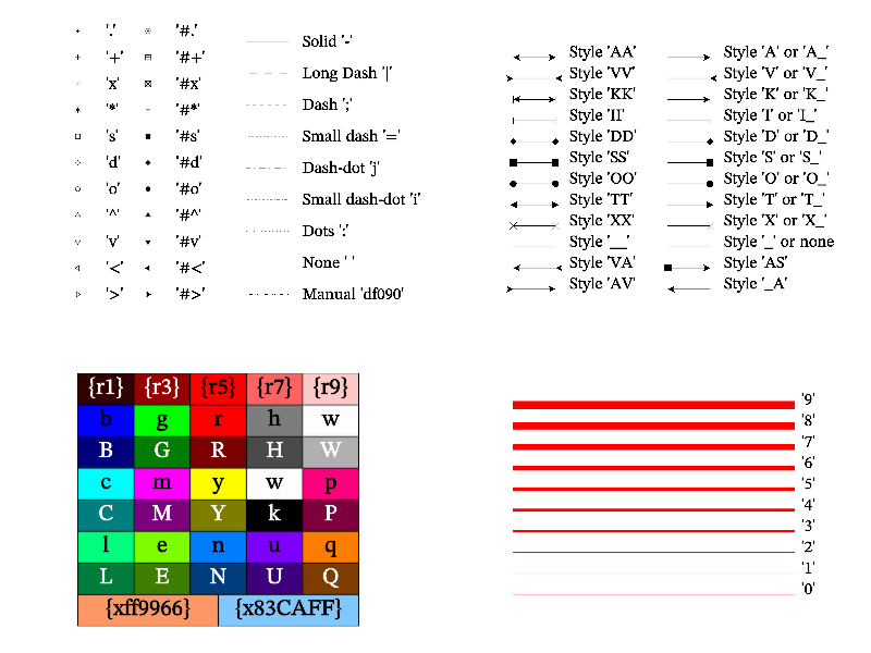
Next: Font styles, Previous: Line styles, Up: General concepts [Contents][Index]
The color scheme is used for determining the color of surfaces, isolines, isosurfaces and so on. The color scheme is defined by the string, which may contain several characters that are color id (see Line styles) or characters ‘#:|’. Symbol ‘#’ switches to mesh drawing or to a wire plot. Symbol ‘|’ disables color interpolation in color scheme, which can be useful, for example, for sharp colors during matrix plotting. Symbol ‘:’ terminate the color scheme parsing. Following it, the user may put styles for the text, rotation axis for curves/isocontours, and so on. Color scheme may contain up to 32 color values.
The final color is a linear interpolation of color array. The color array is constructed from the string ids (including “bright” colors, see Color styles). The argument is the amplitude normalized in color range (see Axis settings). For example, string containing 4 characters ‘bcyr’ corresponds to a colorbar from blue (lowest value) through cyan (next value) through yellow (next value) to the red (highest value). String ‘kw’ corresponds to a colorbar from black (lowest value) to white (highest value). String ‘m’ corresponds to a simple magenta color.
The special 2-axis color scheme (like in map plot) can be used if it contain symbol ‘%’. In this case the second direction (alpha channel) is used as second coordinate for colors. At this, up to 4 colors can be specified for corners: {c1,a1}, {c2,a1}, {c1,a2}, {c2,a2}. Here color and alpha ranges are {c1,c2} and {a1,a2} correspondingly. If one specify less than 4 colors then black color is used for corner {c1,a1}. If only 2 colors are specified then the color of their sum is used for corner {c2,a2}.
There are several useful combinations. String ‘kw’ corresponds to the simplest gray color scheme where higher values are brighter. String ‘wk’ presents the inverse gray color scheme where higher value is darker. Strings ‘kRryw’, ‘kGgw’, ‘kBbcw’ present the well-known hot, summer and winter color schemes. Strings ‘BbwrR’ and ‘bBkRr’ allow to view bi-color figure on white or black background, where negative values are blue and positive values are red. String ‘BbcyrR’ gives a color scheme similar to the well-known jet color scheme.
For more precise coloring, you can change default (equidistant) position of colors in color scheme. The format is ‘{CN,pos}’, ‘{CN,pos}’ or ‘{xRRGGBB,pos}’. The position value pos should be in range [0, 1]. Note, that alternative method for fine tuning of the color scheme is using the formula for coloring (see Curved coordinates).

When coloring by coordinate (used in map), the final color is determined by the position of the point in 3d space and is calculated from formula c=x*c[1] + y*c[2]. Here, c[1], c[2] are the first two elements of color array; x, y are normalized to axis range coordinates of the point.
Additionally, MathGL can apply mask to face filling at bitmap rendering. The kind of mask is specified by one of symbols ‘-+=;oOsS~<>jdD*^’ in color scheme. Mask can be rotated by arbitrary angle by command mask or by three predefined values +45, -45 and 90 degree by symbols ‘\/I’ correspondingly. Examples of predefined masks are shown on the figure below.
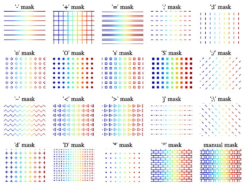
However, you can redefine mask for one symbol by specifying new matrix of size 8*8 as second argument for mask command. For example, the right-down subplot on the figure above is produced by code
gr->SetMask('+', "ff00182424f800"); gr->Dens(a,"3+");
or just use manual mask style (for v.2.3 and later)
gr->Dens(a,"3{s00ff00182424f800}");
Next: Textual formulas, Previous: Color scheme, Up: General concepts [Contents][Index]
Text style is specified by the string which may contain: color id characters ‘wkrgbcymhRGBCYMHW’ (see Color styles), and font style (‘ribwou’) and/or alignment (‘LRC’) specifications. At this, font style and alignment begin after the separator ‘:’. For example, ‘r:iCb’ sets the bold (‘b’) italic (‘i’) font text aligned at the center (‘C’) and with red color (‘r’). Starting from MathGL v.2.3, you can set not single color for whole text, but use color gradient for printed text (see Color scheme).
The font styles are: ‘r’ – roman (or regular) font, ‘i’ – italic style, ‘b’ – bold style. By default roman roman font is used. The align types are: ‘L’ – align left (default), ‘C’ – align center, ‘R’ – align right, ‘T’ – align under, ‘V’ – align center vertical. Additional font effects are: ‘w’ – wired, ‘o’ – over-lined, ‘u’ – underlined.
Also a parsing of the LaTeX-like syntax is provided. There are commands for the font style changing inside the string (for example, use \b for bold font): \a or \overline – over-lined, \b or \textbf – bold, \i or \textit – italic, \r or \textrm – roman (disable bold and italic attributes), \u or \underline – underlined, \w or \wire – wired, \big – bigger size, @ – smaller size. The lower and upper indexes are specified by ‘_’ and ‘^’ symbols. At this the changed font style is applied only on next symbol or symbols in braces {}. The text in braces {} are treated as single symbol that allow one to print the index of index. For example, compare the strings ‘sin (x^{2^3})’ and ‘sin (x^2^3)’. You may also change text color inside string by command #? or by \color? where ‘?’ is symbolic id of the color (see Color styles). For example, words ‘blue’ and ‘red’ will be colored in the string ‘#b{blue} and \colorr{red} text’. The most of functions understand the newline symbol ‘\n’ and allows to print multi-line text. Finally, you can use arbitrary (if it was defined in font-face) UTF codes by command \utf0x????. For example, \utf0x3b1 will produce
α symbol.
The most of commands for special TeX or AMSTeX symbols, the commands for font style changing (\textrm, \textbf, \textit, \textsc, \overline, \underline), accents (\hat, \tilde, \dot, \ddot, \acute, \check, \grave, \bar, \breve) and roots (\sqrt, \sqrt3, \sqrt4) are recognized. The full list contain approximately 2000 commands. Note that first space symbol after the command is ignored, but second one is printed as normal symbol (space). For example, the following strings produce the same result \tilde a: ‘\tilde{a}’; ‘\tilde a’; ‘\tilde{}a’.
In particular, the Greek letters are recognizable special symbols: α – \alpha, β – \beta, γ – \gamma, δ – \delta, ε – \epsilon, η – \eta, ι – \iota, χ – \chi, κ – \kappa, λ – \lambda, μ – \mu, ν – \nu, o – \o, ω – \omega, ϕ – \phi, π – \pi, ψ – \psi, ρ – \rho, σ – \sigma, θ – \theta, τ – \tau, υ – \upsilon, ξ – \xi, ζ – \zeta, ς – \varsigma, ɛ – \varepsilon, ϑ – \vartheta, φ – \varphi, ϰ – \varkappa; A – \Alpha, B – \Beta, Γ – \Gamma, Δ – \Delta, E – \Epsilon, H – \Eta, I – \Iota, C – \Chi, K – \Kappa, Λ – \Lambda, M – \Mu, N – \Nu, O – \O, Ω – \Omega, Φ – \Phi, Π – \Pi, Ψ – \Psi, R – \Rho, Σ – \Sigma, Θ – \Theta, T – \Tau, Υ – \Upsilon, Ξ – \Xi, Z – \Zeta.The small part of most common special TeX symbols are: ∠ – \angle, ⋅ – \cdot, ♣ – \clubsuit, ✓ – \checkmark, ∪ – \cup, ∩ – \cap, ♢ – \diamondsuit, ◇ – \diamond, ÷ – \div, ↓ – \downarrow, † – \dag, ‡ – \ddag, ≡ – \equiv, ∃ – \exists, ⌢ – \frown, ♭ – \flat, ≥ – \ge, ≥ – \geq, ≧ – \geqq, ← – \gets, ♡ – \heartsuit, ∞ – \infty, ∫ – \int, \Int, ℑ – \Im, ♢ – \lozenge, ⟨ – \langle, ≤ – \le, ≤ – \leq, ≦ – \leqq, ← – \leftarrow, ∓ – \mp, ∇ – \nabla, ≠ – \ne, ≠ – \neq, ♮ – \natural, ∮ – \oint, ⊙ – \odot, ⊕ – \oplus, ∂ – \partial, ∥ – \parallel, ⊥ –\perp, ± – \pm, ∝ – \propto, ∏ – \prod, ℜ – \Re, → – \rightarrow, ⟩ – \rangle, ♠ – \spadesuit, ~ – \sim, ⌣ – \smile, ⊂ – \subset, ⊃ – \supset, √ – \sqrt or \surd, § – \S, ♯ – \sharp, ∑ – \sum, × – \times, → – \to, ∴ – \therefore, ↑ – \uparrow, ℘ – \wp.
The font size can be defined explicitly (if size>0) or relatively to a base font size as |size|*FontSize (if size<0). The value size=0 specifies that the string will not be printed. The base font size is measured in internal “MathGL” units. Special functions SetFontSizePT(), SetFontSizeCM(), SetFontSizeIN() (see Font settings) allow one to set it in more “common” variables for a given dpi value of the picture.
Next: Command options, Previous: Font styles, Up: General concepts [Contents][Index]
MathGL have the fast variant of textual formula evaluation (see Evaluate expression) . There are a lot of functions and operators available. The operators are: ‘+’ – addition, ‘-’ – subtraction, ‘*’ – multiplication, ‘/’ – division, ‘%’ – modulo, ‘^’ – integer power. Also there are logical “operators”: ‘<’ – true if x<y, ‘>’ – true if x>y, ‘=’ – true if x=y, ‘&’ – true if x and y both nonzero, ‘|’ – true if x or y nonzero. These logical operators have lowest priority and return 1 if true or 0 if false.
The basic functions are: ‘sqrt(x)’ – square root of x, ‘pow(x,y)’ – power x in y, ‘ln(x)’ – natural logarithm of x, ‘lg(x)’ – decimal logarithm of x, ‘log(a,x)’ – logarithm base a of x, ‘abs(x)’ – absolute value of x, ‘sign(x)’ – sign of x, ‘mod(x,y)’ – x modulo y, ‘step(x)’ – step function, ‘int(x)’ – integer part of x, ‘rnd’ – random number, ‘random(x)’ – random data of size as in x, ‘hypot(x,y)’=sqrt(x^2+y^2) – hypotenuse, ‘cmplx(x,y)’=x+i*y – complex number, ‘pi’ – number π = 3.1415926…, inf=∞
Functions for complex numbers ‘real(x)’, ‘imag(x)’, ‘abs(x)’, ‘arg(x)’, ‘conj(x)’.
Trigonometric functions are: ‘sin(x)’, ‘cos(x)’, ‘tan(x)’ (or ‘tg(x)’). Inverse trigonometric functions are: ‘asin(x)’, ‘acos(x)’, ‘atan(x)’. Hyperbolic functions are: ‘sinh(x)’ (or ‘sh(x)’), ‘cosh(x)’ (or ‘ch(x)’), ‘tanh(x)’ (or ‘th(x)’). Inverse hyperbolic functions are: ‘asinh(x)’, ‘acosh(x)’, ‘atanh(x)’.
There are a set of special functions: ‘gamma(x)’ – Gamma function Γ(x) = ∫0∞ tx-1 exp(-t) dt, ‘gamma_inc(x,y)’ – incomplete Gamma function Γ(x,y) = ∫y∞ tx-1 exp(-t) dt, ‘psi(x)’ – digamma function ψ(x) = Γ′(x)/Γ(x) for x≠0, ‘ai(x)’ – Airy function Ai(x), ‘bi(x)’ – Airy function Bi(x), ‘cl(x)’ – Clausen function, ‘li2(x)’ (or ‘dilog(x)’) – dilogarithm Li2(x) = -ℜ∫0xds log(1-s)/s, ‘sinc(x)’ – compute sinc(x) = sin(πx)/(πx) for any value of x, ‘zeta(x)’ – Riemann zeta function ζ(s) = ∑k=1∞k-s for arbitrary s≠1, ‘eta(x)’ – eta function η(s) = (1 - 21-s)ζ(s) for arbitrary s, ‘lp(l,x)’ – Legendre polynomial Pl(x), (|x|≤1, l≥0), ‘w0(x)’ – principal branch of the Lambert W function, ‘w1(x)’ – principal branch of the Lambert W function. Function W(x) is defined to be solution of the equation: W exp(W) = x.
The exponent integrals are: ‘ci(x)’ – Cosine integral Ci(x) = ∫0xdt cos(t)/t, ‘si(x)’ – Sine integral Si(x) = ∫0xdt sin(t)/t, ‘erf(x)’ – error function erf(x) = (2/√π) ∫0xdt exp(-t2) , ‘ei(x)’ – exponential integral Ei(x) = -PV(∫-x∞dt exp(-t)/t) (where PV denotes the principal value of the integral), ‘e1(x)’ – exponential integral E1(x) = ℜ∫1∞dt exp(-xt)/t, ‘e2(x)’ – exponential integral E2(x) = ℜ∫1∞dt exp(-xt)/t2, ‘ei3(x)’ – exponential integral Ei3(x) = ∫0xdt exp(-t3) for x≥0.
Bessel functions are: ‘j(nu,x)’ – regular cylindrical Bessel function of fractional order nu, ‘y(nu,x)’ – irregular cylindrical Bessel function of fractional order nu, ‘i(nu,x)’ – regular modified Bessel function of fractional order nu, ‘k(nu,x)’ – irregular modified Bessel function of fractional order nu.
Elliptic integrals are: ‘ee(k)’ – complete elliptic integral is denoted by E(k) = E(π/2,k), ‘ek(k)’ – complete elliptic integral is denoted by K(k) = F(π/2,k), ‘e(phi,k)’ – elliptic integral E(φ,k) = ∫0φdt √(1 - k2sin2(t)), ‘f(phi,k)’ – elliptic integral F(φ,k) = ∫0φdt 1/√(1 - k2sin2(t))
Jacobi elliptic functions are: ‘sn(u,m)’, ‘cn(u,m)’, ‘dn(u,m)’, ‘sc(u,m)’, ‘sd(u,m)’, ‘ns(u,m)’, ‘cs(u,m)’, ‘cd(u,m)’, ‘nc(u,m)’, ‘ds(u,m)’, ‘dc(u,m)’, ‘nd(u,m)’.
Note, some of these functions are unavailable if MathGL was compiled without GSL support.
There is no difference between lower or upper case in formulas. If argument value lie outside the range of function definition then function returns NaN.
MathGL version 2.5 introduce user-defined functions ‘fn1()...fn9()’ at formula evaluation, which are defined after symbol ‘\’. For example, "fn1(3)\x^_1" will produce "x^3". Also functions ‘sum’, ‘dsum’, ‘prod’ are added at formula evaluation for summation, summation with variable sign and product evaluation. For example, "sum(_i^2,5)" will produce "30"=0+1^2+2^2+3^2+4^2, "dsum(_i^2,5)" will produce "10"=0-1^2+2^2-3^2+4^2, and "prod(1+_i,5)" will produce 5!="120". You can nest them for variables _i,_j,...,_z, like "sum(sum(_j+_i^2,5),5)" will give "200". Also you can use user-defined functions, like "sum(fn1(_i)-fn2(_i),4)\_1^4\_1^3" is the same as "sum(_i^4-_i^3,4)" and will produce "62".
Next: Interfaces, Previous: Textual formulas, Up: General concepts [Contents][Index]
Command options allow the easy setup of the selected plot by changing global settings only for this plot. Each option start from symbol ‘;’. Options work so that MathGL remember the current settings, change settings as it being set in the option, execute function and return the original settings back. So, the options are most usable for plotting functions.
The most useful options are xrange, yrange, zrange. They sets the boundaries for data change. This boundaries are used for automatically filled variables. So, these options allow one to change the position of some plots. For example, in command Plot(y,"","xrange 0.1 0.9"); or plot y; xrange 0.1 0.9 the x coordinate will be equidistantly distributed in range 0.1 ... 0.9. See Using options, for sample code and picture.
The full list of options are:
valSets alpha value (transparency) of the plot. The value should be in range [0, 1]. See also alphadef.
val1 val2Sets boundaries of x coordinate change for the plot. See also xrange.
val1 val2Sets boundaries of y coordinate change for the plot. See also yrange.
val1 val2Sets boundaries of z coordinate change for the plot. See also zrange.
valSets whether to cut or to project the plot points lying outside the bounding box. See also cut.
valWork like meshnum command.
Adds string ’txt’ to internal legend accumulator. The style of described line and mark is taken from arguments of the last 1D plotting command. See also legend.
valSet the value to be used as additional numeric parameter in plotting command.
Previous: Command options, Up: General concepts [Contents][Index]
The MathGL library has interfaces for a set of languages. Most of them are based on the C interface via SWIG tool. There are Python, Java, Octave, Lisp, C#, Guile, Lua, Modula 3, Ocaml, Perl, PHP, Pike, R, Ruby, and Tcl interfaces. Also there is a Fortran interface which has a similar set of functions, but slightly different types of arguments (integers instead of pointers). These functions are marked as [C function].
Some of the languages listed above support classes (like C++ or Python). The name of functions for them is the same as in C++ (see MathGL core and Data processing) and marked like [Method on mglGraph].
Finally, a special command language MGL (see MGL scripts) was written for a faster access to plotting functions. Corresponding scripts can be executed separately (by UDAV, mglconv, mglview and so on) or from the C/C++/Python/... code (see mglParse class).
| • C interface | ||
| • C++ interface |
Next: C++ interface, Up: Interfaces [Contents][Index]
The C interface is a base for many other interfaces. It contains the pure C functions for most of the methods of MathGL classes. In distinction to C++ classes, C functions must have an argument HMGL (for graphics) and/or HMDT (for data arrays), which specifies the object for drawing or manipulating (changing). So, firstly, the user has to create this object by the function mgl_create_*() and has to delete it after the use by function mgl_delete_*().
All C functions are described in the header file #include <mgl2/mgl_cf.h> and use variables of the following types:
HMGL — Pointer to class mglGraph (see MathGL core).
HCDT — Pointer to class const mglDataA (see Data processing) — constant data array.
HMDT — Pointer to class mglData (see Data processing) — data array of real numbers.
HADT — Pointer to class mglDataC (see Data processing) — data array of complex numbers.
HMPR — Pointer to class mglParse (see mglParse class) — MGL script parsing.
HMEX — Pointer to class mglExpr (see Evaluate expression) — textual formulas for real numbers.
HMAX — Pointer to class mglExprC (see Evaluate expression) — textual formulas for complex numbers.
These variables contain identifiers for graphics drawing objects and for the data objects.
Fortran functions/subroutines have the same names as C functions. However, there is a difference. Variable of type HMGL, HMDT must be an integer with sufficient size (integer*4 in the 32-bit operating system or integer*8 in the 64-bit operating system). All C functions of type void are subroutines in Fortran, which are called by operator call. The exceptions are functions, which return variables of types HMGL or HMDT. These functions should be declared as integer in Fortran code. Also, one should keep in mind that strings in Fortran are denoted by ' symbol, not the " symbol.
Previous: C interface, Up: Interfaces [Contents][Index]
MathGL provides the interface to a set of languages via SWIG library. Some of these languages support classes. The typical example is Python – which is named in this chapter’s title. Exactly the same classes are used for high-level C++ API. Its feature is using only inline member-functions what make high-level API to be independent on compiler even for binary build.
There are 3 main classes in:
mglGraph
– provide most plotting functions (see MathGL core).
mglData
– provide base data processing (see Data processing). It have an additional feature to access data values. You can use a construct like this: dat[i]=sth; or sth=dat[i] where flat representation of data is used (i.e., i can be in range 0...nx*nx*nz-1). You can also import NumPy arrays as input arguments in Python: mgl_dat = mglData(numpy_dat);.
mglParse
– provide functions for parsing MGL scripts (see MGL scripts).
To use Python classes just execute ‘import mathgl’. The simplest example will be:
import mathgl
a=mathgl.mglGraph()
a.Box()
a.WritePNG("test.png")
Alternatively you can import all classes from mathgl module and easily access MathGL classes like this:
from mathgl import *
a=mglGraph()
a.Box()
a.WritePNG("test.png")
This becomes useful if you create many mglData objects, for example.
Next: Widget classes, Previous: General concepts, Up: Top [Contents][Index]
The core of MathGL is mglGraph class defined in #include <mgl2/mgl.h>. It contains a lot of plotting functions for 1D, 2D and 3D data. It also encapsulates parameters for axes drawing. Moreover an arbitrary coordinate transformation can be used for each axis. All plotting functions use data encapsulated in mglData class (see Data processing) that allows to check sizes of used arrays easily. Also it have many functions for data handling: modify it by formulas, find momentums and distribution (histogram), apply operator (differentiate, integrate, transpose, Fourier and so on), change data sizes (interpolate, squeeze, crop and so on). Additional information about colors, fonts, formula parsing can be found in General concepts and Other classes.
Some of MathGL features will appear only in novel versions. To test used MathGL version you can use following function.
mglGraph: bool CheckVersion (const char *ver) staticint mgl_check_version (const char *ver)Return zero if MathGL version is appropriate for required by ver, i.e. if major version is the same and minor version is greater or equal to one in ver.
Next: Graphics setup, Up: MathGL core [Contents][Index]
mglGraph: mglGraph (int kind=0, int width=600, int height=400)mglGraph: mglGraph (const mglGraph &gr)mglGraph: mglGraph (HMGL gr)HMGL mgl_create_graph (int width, int height)HMGL mgl_create_graph_gl ()Creates the instance of class mglGraph with specified sizes width and height. Parameter kind may have following values: ‘0’ – use default plotter, ‘1’ – use OpenGL plotter.
mglGraph: ~mglGraph ()HMGL mgl_delete_graph (HMGL gr)Deletes the instance of class mglGraph.
mglGraph: HMGL Self ()Returns the pointer to internal object of type HMGL.
HMGL mgl_default_graph ()Returns pointer to default instance of class mglGraph. This is default instance, used with new classes, which can be used to keep plot settings and to speed up initialization in small different plots.
Next: Axis settings, Previous: Constructor, Up: MathGL core [Contents][Index]
Functions and variables in this group influences on overall graphics appearance. So all of them should be placed before any actual plotting function calls.
mglGraph: void DefaultPlotParam ()void mgl_set_def_param (HMGL gr)Restore initial values for all of parameters and clear the image.
val flagmglGraph: void SetFlagAdv (int val, uint32_t flag)void mgl_set_flag (HMGL gr, int val, uint32_t flag)Sets the value of internal binary flag to val. The list of flags can be found at define.h. The current list of flags are:
#define MGL_ENABLE_CUT		0x00000004 	///< Flag which determines how points outside bounding box are drown.
#define MGL_ENABLE_RTEXT 	0x00000008 	///< Use text rotation along axis
#define MGL_AUTO_FACTOR		0x00000010 	///< Enable autochange PlotFactor
#define MGL_ENABLE_ALPHA 	0x00000020 	///< Flag that Alpha is used
#define MGL_ENABLE_LIGHT 	0x00000040 	///< Flag of using lightning
#define MGL_TICKS_ROTATE 	0x00000080 	///< Allow ticks rotation
#define MGL_TICKS_SKIP		0x00000100 	///< Allow ticks rotation
#define MGL_DISABLE_SCALE	0x00000200 	///< Temporary flag for disable scaling (used for axis)
#define MGL_FINISHED 		0x00000400 	///< Flag that final picture (i.e. mglCanvas::G) is ready
#define MGL_USE_GMTIME		0x00000800 	///< Use gmtime instead of localtime
#define MGL_SHOW_POS		0x00001000 	///< Switch to show or not mouse click position
#define MGL_CLF_ON_UPD		0x00002000 	///< Clear plot before Update()
#define MGL_NOSUBTICKS		0x00004000 	///< Disable subticks drawing (for bounding box)
#define MGL_LOCAL_LIGHT		0x00008000 	///< Keep light sources for each inplot
#define MGL_VECT_FRAME		0x00010000 	///< Use DrwDat to remember all data of frames
#define MGL_REDUCEACC		0x00020000 	///< Reduce accuracy of points (to reduce size of output files)
#define MGL_PREFERVC 		0x00040000 	///< Prefer vertex color instead of texture if output format supports
#define MGL_ONESIDED 		0x00080000 	///< Render only front side of surfaces if output format supports (for debugging)
#define MGL_NO_ORIGIN 		0x00100000 	///< Don't draw tick labels at axis origin
#define MGL_GRAY_MODE 		0x00200000 	///< Convert all colors to gray ones
#define MGL_FULL_CURV 		0x00400000 	///< Disable omitting points in straight-line part(s)
#define MGL_NO_SCALE_REL 	0x00800000 	///< Disable font scaling in relative inplots
void mgl_bsize (unsigned bsize)Set buffer size for number of primitives as (1<<bsize)^2. I.e. as 10^12 for bsize=20 or 4*10^9 for bsize=16 (default). NOTE: you set it only once before any plotting. The current value is returned.
| • Transparency | ||
| • Lighting | ||
| • Fog | ||
| • Default sizes | ||
| • Cutting | ||
| • Font settings | ||
| • Palette and colors | ||
| • Masks | ||
| • Error handling | ||
| • Stop drawing |
Next: Lighting, Up: Graphics setup [Contents][Index]
There are several functions and variables for setup transparency. The general function is alpha which switch on/off the transparency for overall plot. It influence only for graphics which created after alpha call (with one exception, OpenGL). Function alphadef specify the default value of alpha-channel. Finally, function transptype set the kind of transparency. See Transparency and lighting, for sample code and picture.
[val=on]mglGraph: void Alpha (bool enable)void mgl_set_alpha (HMGL gr, int enable)Sets the transparency on/off and returns previous value of transparency. It is recommended to call this function before any plotting command. Default value is transparency off.
valmglGraph: void SetAlphaDef (mreal val)void mgl_set_alpha_default (HMGL gr, mreal alpha)Sets default value of alpha channel (transparency) for all plotting functions. Initial value is 0.5.
valmglGraph: void SetTranspType (int type)void mgl_set_transp_type (HMGL gr, int type)Set the type of transparency. Possible values are:
SetAlphaDef(0.3) or less for lamp-like transparency.
See Types of transparency, for sample code and picture..
Next: Fog, Previous: Transparency, Up: Graphics setup [Contents][Index]
There are several functions for setup lighting. The general function is light which switch on/off the lighting for overall plot. It influence only for graphics which created after light call (with one exception, OpenGL). Generally MathGL support up to 10 independent light sources. But in OpenGL mode only 8 of light sources is used due to OpenGL limitations. The position, color, brightness of each light source can be set separately. By default only one light source is active. It is source number 0 with white color, located at top of the plot. See Lighting sample, for sample code and picture.
[val=on]mglGraph: bool Light (bool enable)void mgl_set_light (HMGL gr, int enable)Sets the using of light on/off for overall plot. Function returns previous value of lighting. Default value is lightning off.
num valmglGraph: void Light (int n, bool enable)void mgl_set_light_n (HMGL gr, int n, int enable)Switch on/off n-th light source separately.
num xdir ydir zdir ['col'='w' br=0.5]num xdir ydir zdir xpos ypos zpos ['col'='w' br=0.5 ap=0]mglGraph: void AddLight (int n, mglPoint d, char c='w', mreal bright=0.5, mreal ap=0)mglGraph: void AddLight (int n, mglPoint r, mglPoint d, char c='w', mreal bright=0.5, mreal ap=0)void mgl_add_light (HMGL gr, int n, mreal dx, mreal dy, mreal dz)void mgl_add_light_ext (HMGL gr, int n, mreal dx, mreal dy, mreal dz, char c, mreal bright, mreal ap)void mgl_add_light_loc (HMGL gr, int n, mreal rx, mreal ry, mreal rz, mreal dx, mreal dy, mreal dz, char c, mreal bright, mreal ap)The function adds a light source with identification n in direction d with color c and with brightness bright (which must be in range [0,1]). If position r is specified and isn’t NAN then light source is supposed to be local otherwise light source is supposed to be placed at infinity.
valmglGraph: void SetDiffuse (mreal bright)void mgl_set_difbr (HMGL gr, mreal bright)Set brightness of diffusive light (only for local light sources).
valmglGraph: void SetAmbient (mreal bright=0.5)void mgl_set_ambbr (HMGL gr, mreal bright)Sets the brightness of ambient light. The value should be in range [0,1].
valmglGraph: void AttachLight (bool val)void mgl_set_attach_light (HMGL gr, int val)Set to attach light settings to inplot/subplot. Note, OpenGL and some output formats don’t support this feature.
Next: Default sizes, Previous: Lighting, Up: Graphics setup [Contents][Index]
val [dz=0.25]mglGraph: void Fog (mreal d, mreal dz=0.25)void mgl_set_fog (HMGL gr, mreal d, mreal dz)Function imitate a fog in the plot. Fog start from relative distance dz from view point and its density growths exponentially in depth. So that the fog influence is determined by law ~ 1-exp(-d*z). Here z is normalized to 1 depth of the plot. If value d=0 then the fog is absent. Note, that fog was applied at stage of image creation, not at stage of drawing. See Adding fog, for sample code and picture.
Next: Cutting, Previous: Fog, Up: Graphics setup [Contents][Index]
These variables control the default (initial) values for most graphics parameters including sizes of markers, arrows, line width and so on. As any other settings these ones will influence only on plots created after the settings change.
valmglGraph: void SetBarWidth ( mreal val)void mgl_set_bar_width (HMGL gr, mreal val)Sets relative width of rectangles in bars, barh, boxplot, candle, ohlc. Default value is 0.7.
valmglGraph: void SetMarkSize (mreal val)void mgl_set_mark_size (HMGL gr, mreal val)Sets size of marks for 1D plotting. Default value is 1.
valmglGraph: void SetArrowSize (mreal val)void mgl_set_arrow_size (HMGL gr, mreal val)Sets size of arrows for 1D plotting, lines and curves (see Primitives). Default value is 1.
valmglGraph: void SetMeshNum (int val)void mgl_set_meshnum (HMGL gr, int num)Sets approximate number of lines in mesh, fall, grid2, and also the number of hachures in vect, dew, and the number of cells in cloud, and the number of markers in plot, tens, step, mark, textmark. By default (=0) it draws all lines/hachures/cells/markers.
valmglGraph: void SetFaceNum (int val)void mgl_set_facenum (HMGL gr, int num)Sets approximate number of visible faces. Can be used for speeding up drawing by cost of lower quality. By default (=0) it draws all of them.
mglGraph: void SetPlotId (const char *id)void mgl_set_plotid (HMGL gr, const char *id)Sets default name id as filename for saving (in FLTK window for example).
mglGraph: const char * GetPlotId ()const char * mgl_get_plotid (HMGL gr)long gr, char *out, int len)Gets default name id as filename for saving (in FLTK window for example).
valmglGraph: void SetPenDelta (double val)void mgl_pen_delta (HMGL gr, double val)Changes the blur around lines and text (default is 1). For val>1 the text and lines are more sharped. For val<1 the text and lines are more blurred.
Next: Font settings, Previous: Default sizes, Up: Graphics setup [Contents][Index]
These variables and functions set the condition when the points are excluded (cutted) from the drawing. Note, that a point with NAN value(s) of coordinate or amplitude will be automatically excluded from the drawing. See Cutting sample, for sample code and picture.
valmglGraph: void SetCut (bool val)void mgl_set_cut (HMGL gr, int val)Flag which determines how points outside bounding box are drawn. If it is true then points are excluded from plot (it is default) otherwise the points are projected to edges of bounding box.
x1 y1 z1 x2 y2 z2mglGraph: void SetCutBox (mglPoint p1, mglPoint p1)void mgl_set_cut_box (HMGL gr, mreal x1, mreal y1, mreal z1, mreal x2, mreal y2, mreal z2)Lower and upper edge of the box in which never points are drawn. If both edges are the same (the variables are equal) then the cutting box is empty.
mglGraph: void CutOff (const char *cond)void mgl_set_cutoff (HMGL gr, const char *cond)Sets the cutting off condition by formula cond. This condition determine will point be plotted or not. If value of formula is nonzero then point is omitted, otherwise it plotted. Set argument as "" to disable cutting off condition.
Next: Palette and colors, Previous: Cutting, Up: Graphics setup [Contents][Index]
val=6]Font style for text and labels (see text). Initial style is ’fnt’=’:rC’ give Roman font with centering. Parameter val sets the size of font for tick and axis labels. Default font size of axis labels is 1.4 times large than for tick labels. For more detail, see Font styles.
valmglGraph: void SetRotatedText (bool val)void mgl_set_rotated_text (HMGL gr, int val)Sets to use or not text rotation.
valmglGraph: void SetScaleText (bool val)void mgl_set_scale_text (HMGL gr, int val)Sets to scale text in relative inplot (including columnplot, gridplot, stickplot, shearplot) or not.
valmglGraph: void SetTeXparse (bool val)void mgl_set_tex_parse (HMGL gr, int val)Enables/disables TeX-like command parsing at text output.
mglGraph: void LoadFont (const char *name, const char *path="")void mgl_load_font (HMGL gr, const char *name, const char *path)Load font typeface from path/name. Empty name will load default font.
mglGraph: void SetFontDef (const char *fnt)void mgl_set_font_def (HMGL gr, const char * val)Sets the font specification (see Text printing). Default is ‘rC’ – Roman font centering.
mglGraph: void SetFontSize (mreal val)void mgl_set_font_size (HMGL gr, mreal val)Sets the size of font for tick and axis labels. Default font size of axis labels is 1.4 times large than for tick labels.
mglGraph: void SetFontSizePT (mreal cm, int dpi=72)Set FontSize by size in pt and picture DPI (default is 16 pt for dpi=72).
mglGraph: inline void SetFontSizeCM (mreal cm, int dpi=72)Set FontSize by size in centimeters and picture DPI (default is 0.56 cm = 16 pt).
mglGraph: inline void SetFontSizeIN (mreal cm, int dpi=72)Set FontSize by size in inch and picture DPI (default is 0.22 in = 16 pt).
mglGraph: void CopyFont (mglGraph * from)void mgl_copy_font (HMGL gr, HMGL gr_from)Copy font data from another mglGraph object.
mglGraph: void RestoreFont ()void mgl_restore_font (HMGL gr)Restore font data to default typeface.
mglGraph: void SetDefFont (const char *name, const char *path="") staticvoid mgl_def_font (const char *name, const char *path)Load default font typeface (for all newly created HMGL/mglGraph objects) from path/name.
Next: Masks, Previous: Font settings, Up: Graphics setup [Contents][Index]
mglGraph: void SetPalette (const char *colors)void mgl_set_palette (HMGL gr, const char *colors)Sets the palette as selected colors. Default value is "Hbgrcmyhlnqeup" that corresponds to colors: dark gray ‘H’, blue ‘b’, green ‘g’, red ‘r’, cyan ‘c’, magenta ‘m’, yellow ‘y’, gray ‘h’, blue-green ‘l’, sky-blue ‘n’, orange ‘q’, yellow-green ‘e’, blue-violet ‘u’, purple ‘p’. The palette is used mostly in 1D plots (see 1D plotting) for curves which styles are not specified. Internal color counter will be nullified by any change of palette. This includes even hidden change (for example, by box or axis functions).
mglGraph: void SetDefScheme (const char *sch)void mgl_set_def_sch (HMGL gr, const char *sch)Sets the sch as default color scheme. Default value is "BbcyrR".
mglGraph: void SetColor (char id, mreal r, mreal g, mreal b) staticvoid mgl_set_color (char id, mreal r, mreal g, mreal b)Sets RGB values for color with given id. This is global setting which influence on any later usage of symbol id.
val=on]mglGraph: void Gray (bool enable)void mgl_set_gray (HMGL gr, int enable)Sets the gray-scale mode on/off.
Next: Error handling, Previous: Palette and colors, Up: Graphics setup [Contents][Index]
mglGraph: void SetMask (char id, const char *hex)mglGraph: void SetMask (char id, uint64_t hex)void mgl_set_mask (HMGL gr, const char *hex)void mgl_set_mask_val (HMGL gr, uint64_t hex)Sets new bit matrix hex of size 8*8 for mask with given id. This is global setting which influence on any later usage of symbol id. The predefined masks are (see Color scheme): ‘-’ give lines (0x000000FF00000000), ‘+’ give cross-lines (080808FF08080808), ‘=’ give double lines (0000FF00FF000000), ‘;’ give dash lines (0x0000000F00000000), ‘o’ give circles (0000182424180000), ‘O’ give filled circles (0000183C3C180000), ‘s’ give squares (00003C24243C0000), ‘S’ give solid squares (00003C3C3C3C0000), ‘~’ give waves (0000060990600000), ‘<’ give left triangles (0060584658600000), ‘>’ give right triangles (00061A621A060000), ‘j’ give dash-dot lines (0000002700000000), ‘d’ give pluses (0x0008083E08080000), ‘D’ give tacks (0x0139010010931000), ‘*’ give dots (0x0000001818000000), ‘^’ give bricks (0x101010FF010101FF). Parameter angle set the rotation angle too. IMPORTANT: the rotation angle will be replaced by a multiple of 45 degrees at export to EPS.
mglGraph: void SetMaskAngle (int angle)void mgl_set_mask_angle (HMGL gr, int angle)Sets the default rotation angle (in degrees) for masks. Note, you can use symbols ‘\’, ‘/’, ‘I’ in color scheme for setting rotation angles as 45, -45 and 90 degrees correspondingly. IMPORTANT: the rotation angle will be replaced by a multiple of 45 degrees at export to EPS.
Next: Stop drawing, Previous: Masks, Up: Graphics setup [Contents][Index]
Normally user should set it to zero by SetWarn(0); before plotting and check if GetWarn() or Message() return non zero after plotting. Only last warning will be saved. All warnings/errors produced by MathGL is not critical – the plot just will not be drawn. By default, all warnings are printed in stderr. You can disable it by using mgl_suppress_warn(true);.
mglGraph: void SetWarn (int code, const char *info="")void mgl_set_warn (HMGL gr, int code, const char *info)Set warning code. Normally you should call this function only for clearing the warning state, i.e. call SetWarn(0);. Text info will be printed as is if code<0.
mglGraph: const char *Message ()const char *mgl_get_mess (HMGL gr)long gr, char *out, int len)Return messages about matters why some plot are not drawn. If returned string is empty then there are no messages.
mglGraph: int GetWarn ()int mgl_get_warn (HMGL gr)Return the numerical ID of warning about the not drawn plot. Possible values are:
mglWarnNone=0Everything OK
mglWarnDimData dimension(s) is incompatible
mglWarnLowData dimension(s) is too small
mglWarnNegMinimal data value is negative
mglWarnFileNo file or wrong data dimensions
mglWarnMemNot enough memory
mglWarnZeroData values are zero
mglWarnLegNo legend entries
mglWarnSlcSlice value is out of range
mglWarnCntNumber of contours is zero or negative
mglWarnOpenCouldn’t open file
mglWarnLIdLight: ID is out of range
mglWarnSizeSetsize: size(s) is zero or negative
mglWarnFmtFormat is not supported for that build
mglWarnTernAxis ranges are incompatible
mglWarnNullPointer is NULL
mglWarnSpcNot enough space for plot
mglScrArgWrong argument(s) of a command in MGL script
mglScrCmdWrong command in MGL script
mglScrLongToo long line in MGL script
mglScrStrUnbalanced ’ in MGL script
mglScrTempChange temporary data in MGL script
mglGraph: void SuppressWarn (bool state) staticvoid mgl_suppress_warn (int state)Disable printing warnings to stderr if state is nonzero.
mglGraph: void SetGlobalWarn (const char *info) staticvoid mgl_set_global_warn (const char *info)Set warning message info for global scope.
mglGraph: const char * GlobalWarn () staticconst char * mgl_get_global_warn ()Get warning message(s) for global scope.
mglGraph: void ClearGlobalWarn () staticvoid mgl_clear_global_warn ()Clears global warning messages.
Previous: Error handling, Up: Graphics setup [Contents][Index]
mglGraph: void Stop (bool stop=true)void mgl_ask_stop (HMGL gr, int stop)Ask to stop drawing if stop is non-zero, otherwise reset stop flag.
mglGraph: bool NeedStop ()void mgl_need_stop (HMGL gr)Return true if drawing should be terminated. Also it process all events in GUI. User should call this function from time to time inside a long calculation to allow processing events for GUI.
mglGraph: bool SetEventFunc (void (*func)(void *), void *par=NULL)void mgl_set_event_func (HMGL gr, void (*func)(void *), void *par)Set callback function which will be called to process events of GUI library.
Next: Subplots and rotation, Previous: Graphics setup, Up: MathGL core [Contents][Index]
These large set of variables and functions control how the axis and ticks will be drawn. Note that there is 3-step transformation of data coordinates are performed. Firstly, coordinates are projected if Cut=true (see Cutting), after it transformation formulas are applied, and finally the data was normalized in bounding box. Note, that MathGL will produce warning if axis range and transformation formulas are not compatible.
| • Ranges (bounding box) | ||
| • Curved coordinates | ||
| • Ticks |
Next: Curved coordinates, Up: Axis settings [Contents][Index]
v1 v2 [add=off]v1 v2 [add=off]v1 v2 [add=off]v1 v2 [add=off]mglGraph: void SetRange (char dir, mreal v1, mreal v2)mglGraph: void AddRange (char dir, mreal v1, mreal v2)void mgl_set_range_val (HMGL gr, char dir, mreal v1, mreal v2)void mgl_add_range_val (HMGL gr, char dir, mreal v1, mreal v2)Sets or adds the range for ‘x’-,‘y’-,‘z’- coordinate or coloring (‘c’). If one of values is NAN then it is ignored. See also ranges.
add=off]add=off]add=off]add=off]mglGraph: void SetRange (char dir, const mglDataA &dat, bool add=false)void mgl_set_range_dat (HMGL gr, char dir, const HCDT a, int add)Sets the range for ‘x’-,‘y’-,‘z’- coordinate or coloring (‘c’) as minimal and maximal values of data dat. Parameter add=on shows that the new range will be joined to existed one (not replace it).
x1 x2 y1 y2 [z1=0 z2=0]mglGraph: void SetRanges (mglPoint p1, mglPoint p2)mglGraph: void SetRanges (double x1, double x2, double y1, double y2, double z1=0, double z2=0)void mgl_set_ranges (HMGL gr, double x1, double x2, double y1, double y2, double z1, double z2)Sets the ranges of coordinates. If minimal and maximal values of the coordinate are the same then they are ignored. Also it sets the range for coloring (analogous to crange z1 z2). This is default color range for 2d plots. Initial ranges are [-1, 1].
xx yy [zz cc=zz]mglGraph: void SetRanges (const mglDataA &xx, const mglDataA &yy)mglGraph: void SetRanges (const mglDataA &xx, const mglDataA &yy, const mglDataA &zz)mglGraph: void SetRanges (const mglDataA &xx, const mglDataA &yy, const mglDataA &zz, const mglDataA &cc)Sets the ranges of ‘x’-,‘y’-,‘z’-,‘c’-coordinates and coloring as minimal and maximal values of data xx, yy, zz, cc correspondingly.
mglGraph: void SetAutoRanges (mglPoint p1, mglPoint p2)mglGraph: void SetAutoRanges (double x1, double x2, double y1, double y2, double z1=0, double z2=0, double c1=0, double c2=0)void mgl_set_auto_ranges (HMGL gr, double x1, double x2, double y1, double y2, double z1, double z2, double z1, double z2)Sets the ranges for automatic coordinates. If minimal and maximal values of the coordinate are the same then they are ignored.
x0 y0 [z0=nan]mglGraph: void SetOrigin (mglPoint p0)mglGraph: void SetOrigin (mreal x0, mreal y0, mreal z0=NAN)void mgl_set_origin (HMGL gr, mreal x0, mreal y0, mreal z0)Sets center of axis cross section. If one of values is NAN then MathGL try to select optimal axis position.
x1 x2x1 y1 x2 y2x1 y1 z1 x2 y2 z2x1 y1 z1 c1 x2 y2 z2 c2mglGraph: void ZoomAxis (mglPoint p1, mglPoint p2)void mgl_zoom_axis (HMGL gr, mreal x1, mreal y1, mreal z1, mreal c1, mreal x2, mreal y2, mreal z2, mreal c2)Additionally extend axis range for any settings made by SetRange or SetRanges functions according the formula min += (max-min)*p1 and max += (max-min)*p1 (or min *= (max/min)^p1 and max *= (max/min)^p1 for log-axis range when inf>max/min>100 or 0<max/min<0.01). Initial ranges are [0, 1]. Attention! this settings can not be overwritten by any other functions, including DefaultPlotParam().
valmglGraph: void SetFastCut (bool val=true)Enable/disable accurate but slower primitive cutting at axis borders. In C/Fortran you can use mgl_set_flag(gr,val, MGL_FAST_PRIM);. It automatically set on for ternary axis now.
Next: Ticks, Previous: Ranges (bounding box), Up: Axis settings [Contents][Index]
mglGraph: void SetFunc (const char *EqX, const char *EqY, const char *EqZ="", const char *EqA="")void mgl_set_func (HMGL gr, const char *EqX, const char *EqY, const char *EqZ, const char *EqA)Sets transformation formulas for curvilinear coordinate. Each string should contain mathematical expression for real coordinate depending on internal coordinates ‘x’, ‘y’, ‘z’ and ‘a’ or ‘c’ for colorbar. For example, the cylindrical coordinates are introduced as SetFunc("x*cos(y)", "x*sin(y)", "z");. For removing of formulas the corresponding parameter should be empty or NULL. Using transformation formulas will slightly slowing the program. Parameter EqA set the similar transformation formula for color scheme. See Textual formulas.
howmglGraph: void SetCoor (int how)void mgl_set_coor (HMGL gr, int how)Sets one of the predefined transformation formulas for curvilinear coordinate. Parameter how define the coordinates:
mglCartesian=0Cartesian coordinates (no transformation, {x,y,z});
mglPolar=1Polar coordinates: {x*cos(y), x*sin(y), z};
mglSpherical=2Sperical coordinates: {x*sin(y)*cos(z), x*sin(y)*sin(z), x*cos(y)};
mglParabolic=3Parabolic coordinates: {x*y, (x*x-y*y)/2, z}
mglParaboloidal=4Paraboloidal coordinates: {(x*x-y*y)*cos(z)/2, (x*x-y*y)*sin(z)/2, x*y};
mglOblate=5Oblate coordinates: {cosh(x)*cos(y)*cos(z), cosh(x)*cos(y)*sin(z), sinh(x)*sin(y)};
mglProlate=6Prolate coordinates: {sinh(x)*sin(y)*cos(z), sinh(x)*sin(y)*sin(z), cosh(x)*cos(y)};
mglElliptic=7Elliptic coordinates: {cosh(x)*cos(y), sinh(x)*sin(y), z};
mglToroidal=8Toroidal coordinates: {sinh(x)*cos(z)/(cosh(x)-cos(y)), sinh(x)*sin(z)/(cosh(x)-cos(y)), sin(y)/(cosh(x)-cos(y))};
mglBispherical=9Bispherical coordinates: {sin(y)*cos(z)/(cosh(x)-cos(y)), sin(y)*sin(z)/(cosh(x)-cos(y)), sinh(x)/(cosh(x)-cos(y))};
mglBipolar=10Bipolar coordinates: {sinh(x)/(cosh(x)-cos(y)), sin(y)/(cosh(x)-cos(y)), z};
mglLogLog=11Log-log coordinates: {lg(x), lg(y), lg(z)};
mglLogX=12Log-x coordinates: {lg(x), y, z};
mglLogY=13Log-y coordinates: {x, lg(y), z}.
valmglGraph: void Ternary (int tern)void mgl_set_ternary (HMGL gr, int tern)The function sets to draws Ternary (tern=1), Quaternary (tern=2) plot or projections (tern=4,5,6).
Ternary plot is special plot for 3 dependent coordinates (components) a, b, c so that a+b+c=1. MathGL uses only 2 independent coordinates a=x and b=y since it is enough to plot everything. At this third coordinate z act as another parameter to produce contour lines, surfaces and so on.
Correspondingly, Quaternary plot is plot for 4 dependent coordinates a, b, c and d so that a+b+c+d=1. MathGL uses only 3 independent coordinates a=x, b=y and d=z since it is enough to plot everything.
Projections can be obtained by adding value 4 to tern argument. So, that tern=4 will draw projections in Cartesian coordinates, tern=5 will draw projections in Ternary coordinates, tern=6 will draw projections in Quaternary coordinates. If you add 8 instead of 4 then all text labels will not be printed on projections.
Use Ternary(0) for returning to usual axis. See Ternary axis, for sample code and picture. See Axis projection, for sample code and picture.
Previous: Curved coordinates, Up: Axis settings [Contents][Index]
mglGraph: void Adjust (const char *dir="xyzc")void mgl_adjust_ticks (HMGL gr, const char *dir)Set the ticks step, number of sub-ticks and initial ticks position to be the most human readable for the axis along direction(s) dir. Also set SetTuneTicks(true). Usually you don’t need to call this function except the case of returning to default settings.
val [sub=0 org=nan 'fact'='']val [sub=0 org=nan 'fact'='']val [sub=0 org=nan 'fact'='']val sub ['fact'='']val sub ['fact'='']val sub ['fact'='']val ['fact'='']mglGraph: void SetTicks (char dir, mreal d=0, int ns=0, mreal org=NAN, const char *fact="")mglGraph: void SetTicks (char dir, mreal d, int ns, mreal org, const wchar_t *fact)void mgl_set_ticks (HMGL gr, char dir, mreal d, int ns, mreal org)void mgl_set_ticks_fact (HMGL gr, char dir, mreal d, int ns, mreal org, const char *fact)void mgl_set_ticks_factw (HMGL gr, char dir, mreal d, int ns, mreal org, const wchar_t *fact)Set the ticks step d, number of sub-ticks ns (used for positive d) and initial ticks position org for the axis along direction dir (use ’c’ for colorbar ticks). Variable d set step for axis ticks (if positive) or it’s number on the axis range (if negative). Zero value set automatic ticks. If org value is NAN then axis origin is used. Parameter fact set text which will be printed after tick label (like "\pi" for d=M_PI).
val1 'lbl1' [val2 'lbl2' ...]val1 'lbl1' [val2 'lbl2' ...]val1 'lbl1' [val2 'lbl2' ...]val1 'lbl1' [val2 'lbl2' ...]add=off]add=off]add=off]add=off]mglGraph: void SetTicksVal (char dir, const char *lbl, bool add=false)mglGraph: void SetTicksVal (char dir, const wchar_t *lbl, bool add=false)mglGraph: void SetTicksVal (char dir, const mglDataA &val, const char *lbl, bool add=false)mglGraph: void SetTicksVal (char dir, const mglDataA &val, const wchar_t *lbl, bool add=false)void mgl_set_ticks_str (HMGL gr, char dir, const char *lbl, bool add)void mgl_set_ticks_wcs (HMGL gr, char dir, const wchar_t *lbl, bool add)void mgl_set_ticks_val (HMGL gr, char dir, HCDT val, const char *lbl, bool add)void mgl_set_ticks_valw (HMGL gr, char dir, HCDT val, const wchar_t *lbl, bool add)Set the manual positions val and its labels lbl for ticks along axis dir. If array val is absent then values equidistantly distributed in x-axis range are used. Labels are separated by ‘\n’ symbol. If only one value is specified in MGL command then the label will be add to the current ones. Use SetTicks() to restore automatic ticks.
mglGraph: void AddTick (char dir, double val, const char *lbl)mglGraph: void AddTick (char dir, double val, const wchar_t *lbl)void mgl_add_tick (HMGL gr, char dir, double val, const char *lbl)void mgl_set_tickw (HMGL gr, char dir, double val, const wchar_t *lbl)The same as previous but add single tick label lbl at position val to the list of existed ones.
mglGraph: void SetTickTempl (char dir, const char *templ)mglGraph: void SetTickTempl (char dir, const wchar_t *templ)void mgl_set_tick_templ (HMGL gr, const char *templ)void mgl_set_tick_templw (HMGL gr, const wchar_t *templ)Set template templ for x-,y-,z-axis ticks or colorbar ticks. It may contain TeX symbols also. If templ="" then default template is used (in simplest case it is ‘%.2g’). If template start with ‘&’ symbol then long integer value will be passed instead of default type double. Setting on template switch off automatic ticks tuning.
dv=0 'tmpl'='']mglGraph: void SetTicksTime (char dir, mreal val, const char *templ)void mgl_set_ticks_time (HMGL gr, mreal val, const char *templ)Sets time labels with step val and template templ for x-,y-,z-axis ticks or colorbar ticks. It may contain TeX symbols also. The format of template templ is the same as described in http://www.manpagez.com/man/3/strftime/. Most common variants are ‘%X’ for national representation of time, ‘%x’ for national representation of date, ‘%Y’ for year with century. If val=0 and/or templ="" then automatic tick step and/or template will be selected. You can use mgl_get_time() function for obtaining number of second for given date/time string. Note, that MS Visual Studio couldn’t handle date before 1970.
double mgl_get_time (const char*str, const char *templ)Gets number of seconds from 1970 year to specified date/time str. The format of string is specified by templ, which is the same as described in http://www.manpagez.com/man/3/strftime/. Most common variants are ‘%X’ for national representation of time, ‘%x’ for national representation of date, ‘%Y’ for year with century. Note, that MS Visual Studio couldn’t handle date before 1970.
val [pos=1.15]mglGraph: void SetTuneTicks (int tune, mreal pos=1.15)void mgl_tune_ticks (HMGL gr, int tune, mreal pos)Switch on/off ticks enhancing by factoring common multiplier (for small, like from 0.001 to 0.002, or large, like from 1000 to 2000, coordinate values – enabled if tune&1 is nonzero) or common component (for narrow range, like from 0.999 to 1.000 – enabled if tune&2 is nonzero). Also set the position pos of common multiplier/component on the axis: =0 at minimal axis value, =1 at maximal axis value. Default value is 1.15.
dx [dy=0 dz=0 dc=0]mglGraph: void SetTickShift (mglPoint d)void mgl_set_tick_shift (HMGL gr, mreal dx, mreal dy, mreal dz, mreal dc)Set value of additional shift for ticks labels.
mglGraph: void SetTickRotate (bool val)void mgl_set_tick_rotate (HMGL gr, bool val)Enable/disable ticks rotation if there are too many ticks or ticks labels are too long.
mglGraph: void SetTickSkip (bool val)void mgl_set_tick_skip (HMGL gr, bool val)Enable/disable ticks skipping if there are too many ticks or ticks labels are too long.
mglGraph: void SetTimeUTC (bool val)Enable/disable using UTC time for ticks labels. In C/Fortran you can use mgl_set_flag(gr,val, MGL_USE_GMTIME);.
valmglGraph: void SetOriginTick (bool val=true)Enable/disable drawing of ticks labels at axis origin. In C/Fortran you can use mgl_set_flag(gr,val, MGL_NO_ORIGIN);.
val [stt=1]mglGraph: void SetTickLen (mreal val, mreal stt=1)void mgl_set_tick_len (HMGL gr, mreal val, mreal stt)The relative length of axis ticks. Default value is 0.1. Parameter stt>0 set relative length of subticks which is in sqrt(1+stt) times smaller.
mglGraph: void SetAxisStl (const char *stl="k", const char *tck=0, const char *sub=0)void mgl_set_axis_stl (HMGL gr, const char *stl, const char *tck, const char *sub)The line style of axis (stl), ticks (tck) and subticks (sub). If stl is empty then default style is used (‘k’ or ‘w’ depending on transparency type). If tck or sub is empty then axis style is used (i.e. stl).
Next: Export picture, Previous: Axis settings, Up: MathGL core [Contents][Index]
These functions control how and where further plotting will be placed. There is a certain calling order of these functions for the better plot appearance. First one should be subplot, multiplot or inplot for specifying the place. Second one can be title for adding title for the subplot. After it a rotate, shear and aspect. And finally any other plotting functions may be called. Alternatively you can use columnplot, gridplot, stickplot, shearplot or relative inplot for positioning plots in the column (or grid, or stick) one by another without gap between plot axis (bounding boxes). See Subplots, for sample code and picture.
nx ny m ['stl'='<>_^' dx=0 dy=0]mglGraph: void SubPlot (int nx, int ny, int m, const char *stl="<>_^", mreal dx=0, mreal dy=0)void mgl_subplot (HMGL gr, int nx, int ny, int m, const char *stl)void mgl_subplot_d (HMGL gr, int nx, int ny, int m, const char *stl, mreal dx, mreal dy)Puts further plotting in a m-th cell of nx*ny grid of the whole frame area. The position of the cell can be shifted from its default position by relative size dx, dy. This function set off any aspects or rotations. So it should be used first for creating the subplot. Extra space will be reserved for axis/colorbar if stl contain:
From the aesthetical point of view it is not recommended to use this function with different matrices in the same frame. Note, colorbar can be invisible (be out of image borders) if you set empty style ‘’.
nx ny m dx dy ['style'='<>_^' sx sy]mglGraph: void MultiPlot (int nx, int ny, int m, int dx, int dy, const char *stl="<>_^")void mgl_multiplot (HMGL gr, int nx, int ny, int m, int dx, int dy, const char *stl)Puts further plotting in a rectangle of dx*dy cells starting from m-th cell of nx*ny grid of the whole frame area. The position of the rectangular area can be shifted from its default position by relative size sx, sy. This function set off any aspects or rotations. So it should be used first for creating subplot. Extra space will be reserved for axis/colorbar if stl contain:
x1 x2 y1 y2 [rel=on]mglGraph: void InPlot (mreal x1, mreal x2, mreal y1, mreal y2, bool rel=true)void mgl_inplot (HMGL gr, mreal x1, mreal x2, mreal y1, mreal y2)void mgl_relplot (HMGL gr, mreal x1, mreal x2, mreal y1, mreal y2)Puts further plotting in some region of the whole frame surface. This function allows one to create a plot in arbitrary place of the screen. The position is defined by rectangular coordinates [x1, x2]*[y1, y2]. The coordinates x1, x2, y1, y2 are normalized to interval [0, 1]. If parameter rel=true then the relative position to current subplot (or inplot with rel=false) is used. This function set off any aspects or rotations. So it should be used first for creating subplot.
num ind [d=0]mglGraph: void ColumnPlot (int num, int ind, mreal d=0)void mgl_columnplot (HMGL gr, int num, int ind)void mgl_columnplot_d (HMGL gr, int num, int ind, mreal d)Puts further plotting in ind-th cell of column with num cells. The position is relative to previous subplot (or inplot with rel=false). Parameter d set extra gap between cells.
nx ny ind [d=0]mglGraph: void GridPlot (int nx, int ny, int ind, mreal d=0)void mgl_gridplot (HMGL gr, int nx, int ny, int ind)void mgl_gridplot_d (HMGL gr, int nx, int ny, int ind, mreal d)Puts further plotting in ind-th cell of nx*ny grid. The position is relative to previous subplot (or inplot with rel=false). Parameter d set extra gap between cells.
num ind tet phimglGraph: void StickPlot (int num, int ind, mreal tet, mreal phi)void mgl_stickplot (HMGL gr, int num, int ind, mreal tet, mreal phi)Puts further plotting in ind-th cell of stick with num cells. At this, stick is rotated on angles tet, phi. The position is relative to previous subplot (or inplot with rel=false).
num ind sx sy [xd yd]mglGraph: void ShearPlot (int num, int ind, mreal sx, mreal sy, mreal xd=1, mreal yd=0)void mgl_shearplot (HMGL gr, int num, int ind, mreal sx, mreal sy, mreal xd, mreal yd)Puts further plotting in ind-th cell of stick with num cells. At this, cell is sheared on values sx, sy. Stick direction is specified be xd and yd. The position is relative to previous subplot (or inplot with rel=false).
size=-2]mglGraph: void Title (const char *txt, const char *stl="", mreal size=-2)mglGraph: void Title (const wchar_t *txt, const char *stl="", mreal size=-2)void mgl_title (HMGL gr, const char *txt, const char *stl, mreal size)void mgl_titlew (HMGL gr, const wchar_t *txt, const char *stl, mreal size)Add text title for current subplot/inplot. Parameter stl can contain:
Parameter size set font size. This function set off any aspects or rotations. So it should be used just after creating subplot. Note, that each call of this command will reserve extra space. So, you need to manually call subplot command after rasterize if you want to combine bitmap and vector graphics.
tetx tetz [tety=0]mglGraph: void Rotate (mreal TetX, mreal TetZ, mreal TetY=0)void mgl_rotate (HMGL gr, mreal TetX, mreal TetZ, mreal TetY)Rotates a further plotting relative to each axis {x, z, y} consecutively on angles TetX, TetZ, TetY.
tet x y zmglGraph: void RotateN (mreal Tet, mreal x, mreal y, mreal z)void mgl_rotate_vector (HMGL gr, mreal Tet, mreal x, mreal y, mreal z)Rotates a further plotting around vector {x, y, z} on angle Tet.
sx symglGraph: void Shear (mreal sx, mreal sy)void mgl_shear (HMGL gr, mreal sx, mreal sy)Shears a further plotting on values sx, sy.
ax ay [az=1]mglGraph: void Aspect (mreal Ax, mreal Ay, mreal Az=1)void mgl_aspect (HMGL gr, mreal Ax, mreal Ay, mreal Az)Defines aspect ratio for the plot. The viewable axes will be related one to another as the ratio Ax:Ay:Az. For the best effect it should be used after rotate function. If Ax is NAN then function try to select optimal aspect ratio to keep equal ranges for x-y axis. At this, Ay will specify proportionality factor, or set to use automatic one if Ay=NAN.
mglGraph: void Push ()void mgl_mat_push (HMGL gr)Push transformation matrix into stack. Later you can restore its current state by Pop() function.
mglGraph: void Pop ()void mgl_mat_pop (HMGL gr)Pop (restore last ’pushed’) transformation matrix into stack.
mglGraph: void SetPlotFactor (mreal val)void mgl_set_plotfactor (HMGL gr, mreal val)Sets the factor of plot size. It is not recommended to set it lower then 1.5. This is some analogue of function Zoom() but applied not to overall image but for each InPlot. Use negative value or zero to enable automatic selection.
There are 3 functions View(), Zoom() and Perspective() which transform whole image. I.e. they act as secondary transformation matrix. They were introduced for rotating/zooming the whole plot by mouse. It is not recommended to call them for picture drawing.
valmglGraph: void Perspective (mreal a)void mgl_perspective (HMGL gr, mreal a)Add (switch on) the perspective to plot. The parameter a = Depth/(Depth+dz) \in [0,1). By default (a=0) the perspective is off.
tetx tetz [tety=0]mglGraph: void View (mreal TetX, mreal TetZ, mreal TetY=0)void mgl_view (HMGL gr, mreal TetX, mreal TetZ, mreal TetY)Rotates a further plotting relative to each axis {x, z, y} consecutively on angles TetX, TetZ, TetY. Rotation is done independently on rotate. Attention! this settings can not be overwritten by DefaultPlotParam(). Use Zoom(0,0,1,1) to return default view.
x1 y1 x2 y2mglGraph (C++, Python): void Zoom (mreal x1, mreal y1, mreal x2, mreal y2)void mgl_set_zoom (HMGL gr, mreal x1, mreal y1, mreal x2, mreal y2)The function changes the scale of graphics that correspond to zoom in/out of the picture. After function call the current plot will be cleared and further the picture will contain plotting from its part [x1,x2]*[y1,y2]. Here picture coordinates x1, x2, y1, y2 changes from 0 to 1. Attention! this settings can not be overwritten by any other functions, including DefaultPlotParam(). Use Zoom(0,0,1,1) to return default view.
Next: Background, Previous: Subplots and rotation, Up: MathGL core [Contents][Index]
Functions in this group save or give access to produced picture. So, usually they should be called after plotting is done.
w hmglGraph: void SetSize (int width, int height, bool clear=true)void mgl_set_size (HMGL gr, int width, int height)void mgl_scale_size (HMGL gr, int width, int height)Sets size of picture in pixels. This function should be called before any other plotting because it completely remove picture contents if clear=true. Function just clear pixels and scale all primitives if clear=false.
factormglGraph: void SetSizeScl (double factor)void mgl_set_size_scl (HMGL gr, double factor)Set factor for width and height in all further calls of setsize. This command is obsolete since v.2.4.2.
val=2]mglGraph: void SetQuality (int val=MGL_DRAW_NORM)void mgl_set_quality (HMGL gr, int val)Sets quality of the plot depending on value val: MGL_DRAW_WIRE=0 – no face drawing (fastest), MGL_DRAW_FAST=1 – no color interpolation (fast), MGL_DRAW_NORM=2 – high quality (normal), MGL_DRAW_HIGH=3 – high quality with 3d primitives (arrows and marks); MGL_DRAW_LMEM=0x4 – direct bitmap drawing (low memory usage); MGL_DRAW_DOTS=0x8 – for dots drawing instead of primitives (extremely fast).
mglGraph: int GetQuality ()int mgl_get_quality (HMGL gr)Gets quality of the plot: MGL_DRAW_WIRE=0 – no face drawing (fastest), MGL_DRAW_FAST=1 – no color interpolation (fast), MGL_DRAW_NORM=2 – high quality (normal), MGL_DRAW_HIGH=3 – high quality with 3d primitives (arrows and marks); MGL_DRAW_LMEM=0x4 – direct bitmap drawing (low memory usage); MGL_DRAW_DOTS=0x8 – for dots drawing instead of primitives (extremely fast).
mglGraph: void StartGroup (const char *name)void mgl_start_group (HMGL gr, const char *name)Starts group definition. Groups contain objects and other groups, they are used to select a part of a model to zoom to or to make invisible or to make semitransparent and so on.
mglGraph: void EndGroup ()void mgl_end_group (HMGL gr)Ends group definition.
| • Export to file | ||
| • Frames/Animation | ||
| • Bitmap in memory | ||
| • Parallelization |
Next: Frames/Animation, Up: Export picture [Contents][Index]
These functions export current view to a graphic file. The filename fname should have appropriate extension. Parameter descr gives the short description of the picture. Just now the transparency is supported in PNG, SVG, OBJ and PRC files.
mglGraph: void WriteFrame (const char *fname="", const char *descr="")void mgl_write_frame (HMGL gr, const char *fname, const char *descr)Exports current frame to a file fname which type is determined by the extension. Parameter descr adds description to file (can be ""). If fname="" then the file ‘frame####.jpg’ is used, where ‘####’ is current frame id and name ‘frame’ is defined by plotid class property.
-1 y2=-1]mglGraph: void SetBBox (int x1=0, int y1=0, int x2=-1, int y2=-1)void mgl_set_bbox (HMGL gr, int x1, int y1, int x2, int y2)Set boundary box for export graphics into 2D file formats. If x2<0 (y2<0) then original image width (height) will be used. If x1<0 or y1<0 or x1>=x2|Width or y1>=y2|Height then cropping will be disabled.
mglGraph: void WritePNG (const char *fname, const char *descr="", int compr="", bool alpha=true)void mgl_write_png (HMGL gr, const char *fname, const char *descr)void mgl_write_png_solid (HMGL gr, const char *fname, const char *descr)Exports current frame to PNG file. Parameter fname specifies the file name, descr adds description to file, alpha gives the transparency type. By default there are no description added and semitransparent image used. This function does nothing if HAVE_PNG isn’t defined during compilation of MathGL library.
mglGraph: void WriteJPEG (const char *fname, const char *descr="")void mgl_write_jpg (HMGL gr, const char *fname, const char *descr)Exports current frame to JPEG file. Parameter fname specifies the file name, descr adds description to file. By default there is no description added. This function does nothing if HAVE_JPEG isn’t defined during compilation of MathGL library.
mglGraph: void WriteGIF (const char *fname, const char *descr="")void mgl_write_gif (HMGL gr, const char *fname, const char *descr)Exports current frame to GIF file. Parameter fname specifies the file name, descr adds description to file. By default there is no description added. This function does nothing if HAVE_GIF isn’t defined during compilation of MathGL library.
mglGraph: void WriteBMP (const char *fname, const char *descr="")void mgl_write_bmp (HMGL gr, const char *fname, const char *descr)Exports current frame to BMP file. Parameter fname specifies the file name, descr adds description to file. There is no compression used.
mglGraph: void WriteTGA (const char *fname, const char *descr="")void mgl_write_tga (HMGL gr, const char *fname, const char *descr)Exports current frame to TGA file. Parameter fname specifies the file name, descr adds description to file. There is no compression used.
mglGraph: void WriteEPS (const char *fname, const char *descr="")void mgl_write_eps (HMGL gr, const char *fname, const char *descr)Exports current frame to EPS file using vector representation. So it is not recommended for the export of large data plot. It is better to use bitmap format (for example PNG or JPEG). However, program has no internal limitations for size of output file. Parameter fname specifies the file name, descr adds description to file. By default there is no description added. If file name is terminated by ‘z’ (for example, ‘fname.eps.gz’) then file will be compressed in gzip format. Note, that EPS format don’t support color interpolation, and the resulting plot will look as you use quality=1 for plotting.
mglGraph: void WriteBPS (const char *fname, const char *descr="")void mgl_write_eps (HMGL gr, const char *fname, const char *descr)Exports current frame to EPS file using bitmap representation. Parameter fname specifies the file name, descr adds description to file. By default there is no description added. If file name is terminated by ‘z’ (for example, ‘fname.eps.gz’) then file will be compressed in gzip format.
mglGraph: void WriteSVG (const char *fname, const char *descr="")void mgl_write_svg (HMGL gr, const char *fname, const char *descr)Exports current frame to SVG (Scalable Vector Graphics) file using vector representation. In difference of EPS format, SVG format support transparency that allows to correctly draw semitransparent plot (like surfa, surf3a or cloud). Note, the output file may be too large for graphic of large data array (especially for surfaces). It is better to use bitmap format (for example PNG or JPEG). However, program has no internal limitations for size of output file. Parameter fname specifies the file name, descr adds description to file (default is file name). If file name is terminated by ‘z’ (for example, ‘fname.svgz’) then file will be compressed in gzip format. Note, that SVG format don’t support color interpolation, and the resulting plot will look as you use quality=1 for plotting.
mglGraph: void WriteTEX (const char *fname, const char *descr="")void mgl_write_tex (HMGL gr, const char *fname, const char *descr)Exports current frame to LaTeX (package Tikz/PGF) file using vector representation. Note, the output file may be too large for graphic of large data array (especially for surfaces). It is better to use bitmap format (for example PNG or JPEG). However, program has no internal limitations for size of output file. Parameter fname specifies the file name, descr adds description to file (default is file name). Note, there is no text scaling now (for example, in subplots), what may produce miss-aligned labels.
mglGraph: void WritePRC (const char *fname, const char *descr="", bool make_pdf=true)void mgl_write_prc (HMGL gr, const char *fname, const char *descr, int make_pdf)Exports current frame to PRC file using vector representation (see http://en.wikipedia.org/wiki/PRC_%28file_format%29). Note, the output file may be too large for graphic of large data array (especially for surfaces). It is better to use bitmap format (for example PNG or JPEG). However, program has no internal limitations for size of output file. Parameter fname specifies the file name, descr adds description to file (default is file name). If parameter make_pdf=true and PDF was enabled at MathGL configure then corresponding PDF file with 3D image will be created.
mglGraph: void WriteOBJ (const char *fname, const char *descr="")void mgl_write_obj (HMGL gr, const char *fname, const char *descr)Exports current frame to OBJ/MTL file using vector representation (see OBJ format for details). Note, the output file may be too large for graphic of large data array (especially for surfaces). It is better to use bitmap format (for example PNG or JPEG). However, program has no internal limitations for size of output file. Parameter fname specifies the file name, descr adds description to file (default is file name).
mglGraph: void WriteXYZ (const char *fname, const char *descr="")void mgl_write_xyz (HMGL gr, const char *fname, const char *descr)Exports current frame to XYZ/XYZL/XYZF files using vector representation (see XYZ format for details). Note, the output file may be too large for graphic of large data array (especially for surfaces). It is better to use bitmap format (for example PNG or JPEG). However, program has no internal limitations for size of output file. Parameter fname specifies the file name, descr adds description to file (default is file name).
mglGraph: void WriteSTL (const char *fname, const char *descr="")void mgl_write_stl (HMGL gr, const char *fname, const char *descr)Exports current frame to STL file using vector representation (see STL format for details). Note, the output file may be too large for graphic of large data array (especially for surfaces). It is better to use bitmap format (for example PNG or JPEG). However, program has no internal limitations for size of output file. Parameter fname specifies the file name, descr adds description to file (default is file name.
mglGraph: void WriteOFF (const char *fname, const char *descr="", bool colored=false)void mgl_write_off (HMGL gr, const char *fname, const char *descr, bool colored)Exports current frame to OFF file using vector representation (see OFF format for details). Note, the output file may be too large for graphic of large data array (especially for surfaces). It is better to use bitmap format (for example PNG or JPEG). However, program has no internal limitations for size of output file. Parameter fname specifies the file name, descr adds description to file (default is file name).
mglGraph: void ShowImage (const char *viewer, bool nowait=false)void mgl_show_image (const char *viewer, int nowait)Displays the current picture using external program viewer for viewing. The function save the picture to temporary file and call viewer to display it. If nowait=true then the function return immediately (it will not wait while window will be closed).
mglGraph: void WriteJSON (const char *fname, const char *descr="")void mgl_write_json (HMGL gr, const char *fname, const char *descr)Exports current frame to textual file using JSON format. Later this file can be used for faster loading and viewing by JavaScript script. Parameter fname specifies the file name, descr adds description to file.
mglGraph: void ExportMGLD (const char *fname, const char *descr="")void mgl_export_mgld (HMGL gr, const char *fname, const char *descr)Exports points and primitives in file using MGLD format. Later this file can be used for faster loading and viewing by mglview utility. Parameter fname specifies the file name, descr adds description to file (default is file name).
mglGraph: void ImportMGLD (const char *fname, bool add=false)void mgl_import_mgld (HMGL gr, const char *fname, int add)Imports points and primitives in file using MGLD format. Later this file can be used for faster loading and viewing by mglview utility. Parameter fname specifies the file name, add sets to append or replace primitives to existed ones.
Next: Bitmap in memory, Previous: Export to file, Up: Export picture [Contents][Index]
These functions provide ability to create several pictures simultaneously. For most of cases it is useless but for widget classes (see Widget classes) they can provide a way to show animation. Also you can write several frames into animated GIF file.
mglGraph: void NewFrame ()void mgl_new_frame (HMGL gr)Creates new frame. Function returns current frame id. This is not thread safe function in OpenGL mode! Use direct list creation in multi-threading drawing. The function EndFrame() must be call after the finishing of the frame drawing for each call of this function.
mglGraph: void EndFrame ()void mgl_end_frame (HMGL gr)Finishes the frame drawing.
mglGraph: int GetNumFrame ()int mgl_get_num_frame (HMGL gr)Gets the number of created frames.
mglGraph: void SetFrame (int i)void mgl_set_frame (HMGL gr, int i)Finishes the frame drawing and sets drawing data to frame i, which should be in range [0, GetNumFrame()-1]. This function is similar to EndFrame() but don’t add frame to the GIF image.
mglGraph: void GetFrame (int i)void mgl_get_frame (HMGL gr, int i)Replaces drawing data by one from frame i. Function work if MGL_VECT_FRAME is set on (by default).
mglGraph: void ShowFrame (int i)void mgl_show_frame (HMGL gr, int i)Appends drawing data from frame i to current one. Function work if MGL_VECT_FRAME is set on (by default).
mglGraph: void DelFrame (int i)void mgl_del_frame (HMGL gr, int i)Deletes drawing data for frame i and shift all later frame indexes. Function work if MGL_VECT_FRAME is set on (by default). Do nothing in OpenGL mode.
mglGraph: void ResetFrames ()void mgl_reset_frames (HMGL gr)Reset frames counter (start it from zero).
mglGraph: void ClearFrame (int i)void mgl_clear_frame (HMGL gr, int i)Clear list of primitives for current drawing.
mglGraph: void StartGIF (const char *fname, int ms=100)void mgl_start_gif (HMGL gr, const char *fname, int ms)Start writing frames into animated GIF file fname. Parameter ms set the delay between frames in milliseconds. You should not change the picture size during writing the cinema. Use CloseGIF() to finalize writing. Note, that this function is disabled in OpenGL mode.
mglGraph: void CloseGIF ()void mgl_close_gif (HMGL gr)Finish writing animated GIF and close connected pointers.
Next: Parallelization, Previous: Frames/Animation, Up: Export picture [Contents][Index]
These functions return the created picture (bitmap), its width and height. You may display it by yourself in any graphical library (see also, Widget classes) or save in file (see also, Export to file).
mglGraph: const unsigned char * GetRGB ()mglGraph: void GetRGB (char *buf, int size)mglGraph: void GetBGRN (char *buf, int size)const unsigned char * mgl_get_rgb (HMGL gr)Gets RGB bitmap of the current state of the image. Format of each element of bits is: {red, green, blue}. Number of elements is Width*Height. Position of element {i,j} is [3*i + 3*Width*j] (or is [4*i + 4*Width*j] for GetBGRN()). You have to provide the proper size of the buffer, buf, i.e. the code for Python should look like
from mathgl import *
gr = mglGraph();
bits='\t';
bits=bits.expandtabs(4*gr.GetWidth()*gr.GetHeight());
gr.GetBGRN(bits, len(bits));
mglGraph: const unsigned char * GetRGBA ()mglGraph: void GetRGBA (char *buf, int size)const unsigned char * mgl_get_rgba (HMGL gr)Gets RGBA bitmap of the current state of the image. Format of each element of bits is: {red, green, blue, alpha}. Number of elements is Width*Height. Position of element {i,j} is [4*i + 4*Width*j].
mglGraph: int GetWidth ()mglGraph: int GetHeight ()int mgl_get_width (HMGL gr)int mgl_get_height (HMGL gr)Gets width and height of the image.
mglGraph: mglPoint CalcXYZ (int xs, int ys)void mgl_calc_xyz (HMGL gr, int xs, int ys, mreal *x, mreal *y, mreal *z)Calculate 3D coordinate {x,y,z} for screen point {xs,ys}. At this moment it ignore perspective and transformation formulas (curvilinear coordinates). The calculation are done for the last used InPlot (see Subplots and rotation).
mglGraph: mglPoint CalcScr (mglPoint p)void mgl_calc_scr (HMGL gr, mreal x, mreal y, mreal z, int *xs, int *ys)Calculate screen point {xs,ys} for 3D coordinate {x,y,z}. The calculation are done for the last used InPlot (see Subplots and rotation).
mglGraph: void SetObjId (int id)void mgl_set_obj_id (HMGL gr, int id)Set the numeric id for object or subplot/inplot.
mglGraph: int GetObjId (int xs, int ys)int mgl_get_obj_id (HMGL gr, int xs, int ys)Get the numeric id for most upper object at pixel {xs, ys} of the picture. Note, that all plots in the same line of MGL script have the same id.
mglGraph: int GetSplId (int xs, int ys)int mgl_get_spl_id (HMGL gr, int xs, int ys)Get the numeric id for most subplot/inplot at pixel {xs, ys} of the picture.
mglGraph: void Highlight (int id)void mgl_highlight (HMGL gr, int id)Highlight the object with given id.
mglGraph: long IsActive (int xs, int ys, int d=1)long mgl_is_active (HMGL gr, int xs, int ys, int d)Checks if point {xs, ys} is close to one of active point (i.e. mglBase::Act) with accuracy d and return its index or -1 if not found. Active points are special points which characterize primitives (like edges and so on). This function for advanced users only.
mglGraph: long SetDrawReg (int nx=1, int ny=1, int m=0)long mgl_set_draw_reg (HMGL gr, int nx, int ny, int m)Limits drawing region by rectangular area of m-th cell of matrix with sizes nx*ny (like in subplot). This function can be used to update only small region of the image for purposes of higher speed. This function for advanced users only.
Previous: Bitmap in memory, Up: Export picture [Contents][Index]
Many of things MathGL do in parallel by default (if MathGL was built with pthread). However, there is function which set the number of threads to be used.
int mgl_set_num_thr (int n)Set the number of threads to be used by MathGL. If n<1 then the number of threads is set as maximal number of processors (cores). If n=1 then single thread will be used (this is default if pthread was disabled).
Another option is combining bitmap image (taking into account Z-ordering) from different instances of mglGraph. This method is most appropriate for computer clusters when the data size is so large that it exceed the memory of single computer node.
mglGraph: int Combine (const mglGraph *g)int mgl_combine_gr (HMGL gr, HMGL g)Combine drawing from instance g with gr (or with this) taking into account Z-ordering of pixels. The width and height of both instances must be the same.
mglGraph: int MPI_Send (int id)int mgl_mpi_send (HMGL gr, int id)Send graphical information from node id using MPI. The width and height in both nodes must be the same.
mglGraph: int MPI_Recv (int id)int mgl_mpi_send (HMGL gr, int id)Receive graphical information from node id using MPI. The width and height in both nodes must be the same.
Next: Primitives, Previous: Export picture, Up: MathGL core [Contents][Index]
These functions change background image.
mglGraph: void Clf ()mglGraph: void Clf (const char * col)mglGraph: void Clf (char col)mglGraph: void Clf (mreal r, mreal g, mreal b)void mgl_clf (HMGL gr)void mgl_clf_str (HMGL gr, const char * col)void mgl_clf_chr (HMGL gr, char col)void mgl_clf_rgb (HMGL gr, mreal r, mreal g, mreal b)void mgl_clf_rgba (HMGL gr, mreal r, mreal g, mreal b, mreal a)Clear the picture and fill background by specified color.
mglGraph: void Rasterize ()void mgl_rasterize (HMGL gr)Force drawing the plot and use it as background. After it, function clear the list of primitives, like clf. This function is useful if you want save part of plot as bitmap one (for example, large surfaces, isosurfaces or vector fields) and keep some parts as vector one (like annotation, curves, axis and so on). Often, you need to manually call subplot command after rasterize to avoid extra space allocation or plot rotation.
alpha=1]alpha=1]mglGraph: void LoadBackground (const char * fname, double alpha=1)void mgl_load_background (HMGL gr, const char * fname, double alpha)mglGraph: void LoadBackground (const char * fname, const char * how, double alpha=1)void mgl_load_background_ext (HMGL gr, const char * fname, const char * how, double alpha)Load PNG or JPEG file fname as background for the plot. Parameter alpha manually set transparency of the background. Parameter how can be: ‘a’ for filling current subplot only, ‘s’ for scaling (resizing) image to whole area, ‘c’ for centering image, ‘m’ for tessellate image as mosaic.
r g bmglGraph: void FillBackground (const mglColor &rgb)void mgl_fill_background (HMGL gr, double r, double g, double b, double a)Fill background by the specified color. Values should be in range [0,1].
Next: Text printing, Previous: Background, Up: MathGL core [Contents][Index]
These functions draw some simple objects like line, point, sphere, drop, cone and so on. See Using primitives, for sample code and picture.
x y ['col'='r.']x y z ['col'='r.']mglGraph: void Ball (mglPoint p, char col='r')mglGraph: void Mark (mglPoint p, const char *mark)void mgl_mark (HMGL gr, mreal x, mreal y, mreal z, const char *mark)Draws a mark (point ‘.’ by default) at position p={x, y, z} with color col.
x y ex ey ['stl'='']x y z ex ey ez ['stl'='']mglGraph: void Error (mglPoint p, mglPoint e, char *stl="")void mgl_error_box (HMGL gr, mreal x, mreal y, mreal z, mreal ex, mreal ey, mreal ez, char *stl)Draws a 3d error box at position p={x, y, z} with sizes e={ex, ey, ez} and style stl. Use NAN for component of e to reduce number of drawn elements.
x1 y1 x2 y2 ['stl'='']x1 y1 z1 x2 y2 z2 ['stl'='']mglGraph: void Line (mglPoint p1, mglPoint p2, char *stl="B", int num=2)void mgl_line (HMGL gr, mreal x1, mreal y1, mreal z1, mreal x2, mreal y2, mreal z2, char *stl, int num)Draws a geodesic line (straight line in Cartesian coordinates) from point p1 to p2 using line style stl. Parameter num define the “quality” of the line. If num=2 then the straight line will be drawn in all coordinate system (independently on transformation formulas (see Curved coordinates). Contrary, for large values (for example, =100) the geodesic line will be drawn in corresponding coordinate system (straight line in Cartesian coordinates, circle in polar coordinates and so on). Line will be drawn even if it lies out of bounding box.
x1 y1 dx1 dy1 x2 y2 dx2 dy2 ['stl'='']x1 y1 z1 dx1 dy1 dz1 x2 y2 z2 dx2 dy2 dz2 ['stl'='']mglGraph: void Curve (mglPoint p1, mglPoint d1, mglPoint p2, mglPoint d2, const char *stl="B", int num=100)void mgl_curve (HMGL gr, mreal x1, mreal y1, mreal z1, mreal dx1, mreal dy1, mreal dz1, mreal x2, mreal y2, mreal z2, mreal dx2, mreal dy2, mreal dz2, const char *stl, int num)Draws Bezier-like curve from point p1 to p2 using line style stl. At this tangent is codirected with d1, d2 and proportional to its amplitude. Parameter num define the “quality” of the curve. If num=2 then the straight line will be drawn in all coordinate system (independently on transformation formulas, see Curved coordinates). Contrary, for large values (for example, =100) the spline like Bezier curve will be drawn in corresponding coordinate system. Curve will be drawn even if it lies out of bounding box.
x1 y1 x2 y2 x3 y3 x4 y4 ['stl'='']x1 y1 z1 x2 y2 z2 x3 y3 z3 x4 y4 z4 ['stl'='']mglGraph: void Face (mglPoint p1, mglPoint p2, mglPoint p3, mglPoint p4, const char *stl="w")void mgl_face (HMGL gr, mreal x1, mreal y1, mreal z1, mreal x2, mreal y2, mreal z2, mreal x3, mreal y3, mreal z3, mreal x4, mreal y4, mreal z4, const char *stl)Draws the solid quadrangle (face) with vertexes p1, p2, p3, p4 and with color(s) stl. At this colors can be the same for all vertexes or different if all 4 colors are specified for each vertex. Face will be drawn even if it lies out of bounding box. Argument stl can also contain mask specification (see Color scheme).
x1 y1 x2 y2 ['stl'='']x1 y1 z1 x2 y2 z2 ['stl'='']Draws the solid rectangle (face) with vertexes {x1, y1, z1} and {x2, y2, z2} with color stl. At this colors can be the same for all vertexes or separately if all 4 colors are specified for each vertex. Face will be drawn even if it lies out of bounding box. Argument stl can also contain mask specification (see Color scheme).
x0 y0 z0 wy wz ['stl'='' d1=0 d2=0]x0 y0 z0 wx wz ['stl'='' d1=0 d2=0]x0 y0 z0 wx wy ['stl'='' d1=0 d2=0]mglGraph: void FaceX (mreal x0, mreal y0, mreal z0, mreal wy, mreal wz, const char *stl="w", mreal d1=0, mreal d2=0)mglGraph: void FaceY (mreal x0, mreal y0, mreal z0, mreal wx, mreal wz, const char *stl="w", mreal d1=0, mreal d2=0)mglGraph: void FaceZ (mreal x0, mreal y0, mreal z0, mreal wx, mreal wy, const char *stl="w", mreal d1=0, mreal d2=0)void mgl_facex (HMGL gr, mreal x0, mreal y0, mreal z0, mreal wy, mreal wz, const char *stl, mreal d1, mreal d2)void mgl_facey (HMGL gr, mreal x0, mreal y0, mreal z0, mreal wx, mreal wz, const char *stl, mreal d1, mreal d2)void mgl_facez (HMGL gr, mreal x0, mreal y0, mreal z0, mreal wx, mreal wy, const char *stl, mreal d1, mreal d2)Draws the solid rectangle (face) perpendicular to [x,y,z]-axis correspondingly at position {x0, y0, z0} with color stl and with widths wx, wy, wz along corresponding directions. At this colors can be the same for all vertexes or separately if all 4 colors are specified for each vertex. Argument stl can also contain mask specification (see Color scheme). Parameters d1!=0, d2!=0 set additional shift of the last vertex (i.e. to draw quadrangle). Face will be drawn even if it lies out of bounding box.
x0 y0 r ['col'='r']x0 y0 z0 r ['col'='r']mglGraph: void Sphere (mglPoint p, mreal r, const char *stl="r")void mgl_sphere (HMGL gr, mreal x0, mreal y0, mreal z0, mreal r, const char *stl)Draw the sphere with radius r and center at point p={x0, y0, z0} and color stl.
x0 y0 dx dy r ['col'='r' sh=1 asp=1]x0 y0 z0 dx dy dz r ['col'='r' sh=1 asp=1]mglGraph: void Drop (mglPoint p, mglPoint d, mreal r, const char *col="r", mreal shift=1, mreal ap=1)void mgl_drop (HMGL gr, mreal x0, mreal y0, mreal z0, mreal dx, mreal dy, mreal dz, mreal r, const char *col, mreal shift, mreal ap)Draw the drop with radius r at point p elongated in direction d and with color col. Parameter shift set the degree of drop oblongness: ‘0’ is sphere, ‘1’ is maximally oblongness drop. Parameter ap set relative width of the drop (this is analogue of “ellipticity” for the sphere).
x1 y1 z1 x2 y2 z2 r1 [r2=-1 'stl'='']mglGraph: void Cone (mglPoint p1, mglPoint p2, mreal r1, mreal r2=-1, const char *stl="B")void mgl_cone (HMGL gr, mreal x1, mreal y1, mreal z1, mreal x2, mreal y2, mreal z2, mreal r1, mreal r2, const char *stl)Draw tube (or truncated cone if edge=false) between points p1, p2 with radius at the edges r1, r2. If r2<0 then it is supposed that r2=r1. The cone color is defined by string stl. Parameter stl can contain:
x0 y0 r ['col'='r']x0 y0 z0 r ['col'='r']mglGraph: void Circle (mglPoint p, mreal r, const char *stl="r")Draw the circle with radius r and center at point p={x0, y0, z0}. Parameter col may contain
x1 y1 x2 y2 r ['col'='r']x1 y1 z1 x2 y2 z2 r ['col'='r']mglGraph: void Ellipse (mglPoint p1, mglPoint p2, mreal r, const char *col="r")void mgl_ellipse (HMGL gr, mreal x1, mreal y1, mreal z1, mreal x2, mreal y2, mreal z2, mreal r, const char *col)Draw the ellipse with radius r and focal points p1, p2. Parameter col may contain
x1 y1 x2 y2 r ['col'='r']x1 y1 z1 x2 y2 z2 r ['col'='r']mglGraph: void Rhomb (mglPoint p1, mglPoint p2, mreal r, const char *col="r")void mgl_rhomb (HMGL gr, mreal x1, mreal y1, mreal z1, mreal x2, mreal y2, mreal z2, mreal r, const char *col)Draw the rhombus with width r and edge points p1, p2. Parameter col may contain
x0 y0 x1 y1 a ['col'='r']x0 y0 z0 x1 y1 a ['col'='r']x0 y0 z0 xa ya za x1 y1 z1 a ['col'='r']mglGraph: void Arc (mglPoint p0, mglPoint p1, mreal a, const char *col="r")mglGraph: void Arc (mglPoint p0, mglPoint pa, mglPoint p1, mreal a, const char *col="r")void mgl_arc (HMGL gr, mreal x0, mreal y0, mreal x1, mreal y1, mreal a, const char *col)void mgl_arc_ext (HMGL gr, mreal x0, mreal y0, mreal z0, mreal xa, mreal ya, mreal za, mreal x1, mreal y1, mreal z1, mreal a, const char *col)Draw the arc around axis pa (default is z-axis pa={0,0,1}) with center at p0 and starting from point p1. Parameter a set the angle of arc in degree. Parameter col may contain color of the arc and arrow style for arc edges.
x0 y0 x1 y1 num ['col'='r']x0 y0 z0 x1 y1 z1 num ['col'='r']mglGraph: void Polygon (mglPoint p0, mglPoint p1, int num, const char *col="r")void mgl_polygon (HMGL gr, mreal x0, mreal y0, mreal z0, mreal x1, mreal y1, mreal z1, int num, const char *col)Draw the polygon with num edges starting from p1. The center of polygon is located in p0. Parameter col may contain
mglGraph: void Logo (const char *fname, bool smooth=false, const char *opt="")mglGraph: void Logo (long w, long h, const unsigned char *rgba, bool smooth=false, const char *opt="")void mgl_logo (HMGL gr, long w, long h, const unsigned char *rgba, bool smooth, const char *opt)void mgl_logo_file (HMGL gr, const char *fname, bool smooth, const char *opt)Draw bitmap (logo) along whole axis range, which can be changed by Command options. Bitmap can be loaded from file or specified as RGBA values for pixels. Parameter smooth set to draw bitmap without or with color interpolation.
x y 'id' ['fnt'='' size=-1]x y z 'id' ['fnt'='' size=-1]mglGraph: void Symbol (mglPoint p, char id, const char *fnt="", mreal size=-1)void mgl_symbol (HMGL gr, mreal x, mreal y, mreal z, char id, const char *fnt, mreal size)Draws user-defined symbol with name id at position p with style specifying by fnt. The size of font is set by size parameter (default is -1). The string fnt may contain color specification ended by ‘:’ symbol; styles ‘a’, ‘A’ to draw at absolute position {x, y} (supposed to be in range [0,1]) of picture (for ‘A’) or subplot/inplot (for ‘a’); and style ‘w’ to draw wired symbol.
x y dx dy 'id' ['fnt'=':L' size=-1]x y z dx dy dz 'id' ['fnt'=':L' size=-1]mglGraph: void Symbol (mglPoint p, mglPoint d, char id, const char *fnt="", mreal size=-1)void mgl_symbol_dir (HMGL gr, mreal x, mreal y, mreal z, mreal dx, mreal dy, mreal dz, const char *text, const char *fnt, mreal size)The same as previous but symbol will be drawn rotated along direction d.
mglGraph: void DefineSymbol (char id, const mglDataA &xdat, const mglDataA &ydat)void mgl_define_symbol (HMGL gr, HCDT xdat, HCDT ydat)Add user-defined symbol with name id and contour {xdat, ydat}. You can use NAN values to set break (jump) of contour curve.
Next: Axis and Colorbar, Previous: Primitives, Up: MathGL core [Contents][Index]
These functions draw the text. There are functions for drawing text in arbitrary place, in arbitrary direction and along arbitrary curve. MathGL can use arbitrary font-faces and parse many TeX commands (for more details see Font styles). All these functions have 2 variant: for printing 8-bit text (char *) and for printing Unicode text (wchar_t *). In first case the conversion into the current locale is used. So sometimes you need to specify it by setlocale() function. The size argument control the size of text: if positive it give the value, if negative it give the value relative to SetFontSize(). The font type (STIX, arial, courier, times and so on) can be selected by function LoadFont(). See Font settings.
The font parameters are described by string. This string may set the text color ‘wkrgbcymhRGBCYMHW’ (see Color styles). Starting from MathGL v.2.3, you can set color gradient for text (see Color scheme). Also, after delimiter symbol ‘:’, it can contain characters of font type (‘rbiwou’) and/or align (‘LRCTV’) specification. The font types are: ‘r’ – roman (or regular) font, ‘i’ – italic style, ‘b’ – bold style, ‘w’ – wired style, ‘o’ – over-lined text, ‘u’ – underlined text. By default roman font is used. The align types are: ‘L’ – align left (default), ‘C’ – align center, ‘R’ – align right, ‘T’ – align under, ‘V’ – align center vertical. For example, string ‘b:iC’ correspond to italic font style for centered text which printed by blue color.
If string contains symbols ‘aA’ then text is printed at absolute position {x, y} (supposed to be in range [0,1]) of picture (for ‘A’) or subplot/inplot (for ‘a’). If string contains symbol ‘@’ then box around text is drawn.
See Text features, for sample code and picture.
x y 'text' ['fnt'='' size=-1]x y z 'text' ['fnt'='' size=-1]mglGraph: void Puts (mglPoint p, const char *text, const char *fnt=":C", mreal size=-1)mglGraph: void Putsw (mglPoint p, const wchar_t *text, const char *fnt=":C", mreal size=-1)mglGraph: void Puts (mreal x, mreal y, const char *text, const char *fnt=":AC", mreal size=-1)mglGraph: void Putsw (mreal x, mreal y, const wchar_t *text, const char *fnt=":AC", mreal size=-1)void mgl_puts (HMGL gr, mreal x, mreal y, mreal z, const char *text, const char *fnt, mreal size)void mgl_putsw (HMGL gr, mreal x, mreal y, mreal z, const wchar_t *text, const char *fnt, mreal size)Draws the string text at position p with fonts specifying by the criteria fnt. The size of font is set by size parameter (default is -1).
x y dx dy 'text' ['fnt'=':L' size=-1]x y z dx dy dz 'text' ['fnt'=':L' size=-1]mglGraph: void Puts (mglPoint p, mglPoint d, const char *text, const char *fnt=":L", mreal size=-1)mglGraph: void Putsw (mglPoint p, mglPoint d, const wchar_t *text, const char *fnt=":L", mreal size=-1)void mgl_puts_dir (HMGL gr, mreal x, mreal y, mreal z, mreal dx, mreal dy, mreal dz, const char *text, const char *fnt, mreal size)void mgl_putsw_dir (HMGL gr, mreal x, mreal y, mreal z, mreal dx, mreal dy, mreal dz, const wchar_t *text, const char *fnt, mreal size)Draws the string text at position p along direction d with specified size. Parameter fnt set text style and text position: under (‘T’) or above (‘t’) the line.
x y 'fname' [n=0 'fnt'='' size=-1.4]x y z 'fname' [n=0 'fnt'='' size=-1.4]Draws unrotated n-th line of file fname at position {x,y,z} with specified size. By default parameters from font command are used.
mglGraph: void Text (const mglDataA &y, const char *text, const char *fnt="", const char *opt="")mglGraph: void Text (const mglDataA &y, const wchar_t *text, const char *fnt="", const char *opt="")mglGraph: void Text (const mglDataA &x, const mglDataA &y, const char *text, const char *fnt="", const char *opt="")mglGraph: void Text (const mglDataA &x, const mglDataA &y, const wchar_t *text, const char *fnt="", const char *opt="")mglGraph: void Text (const mglDataA &x, const mglDataA &y, const mglDataA &z, const char *text, const char *fnt="", const char *opt="")mglGraph: void Text (const mglDataA &x, const mglDataA &y, const mglDataA &z, const wchar_t *text, const char *fnt="", const char *opt="")void mgl_text_y (HMGL gr, HCDT y, const char *text, const char *fnt, const char *opt)void mgl_textw_y (HMGL gr, HCDT y, const wchar_t *text, const char *fnt, const char *opt)void mgl_text_xy (HCDT x, HCDT y, const char *text, const char *fnt, const char *opt)void mgl_textw_xy (HCDT x, HCDT y, const wchar_t *text, const char *fnt, const char *opt)void mgl_text_xyz (HCDT x, HCDT y, HCDT z, const char *text, const char *fnt, const char *opt)void mgl_textw_xyz (HCDT x, HCDT y, HCDT z, const wchar_t *text, const char *fnt, const char *opt)The function draws text along the curve between points {x[i], y[i], z[i]} by font style fnt. The string fnt may contain symbols ‘t’ for printing the text under the curve (default), or ‘T’ for printing the text under the curve. The sizes of 1st dimension must be equal for all arrays x.nx=y.nx=z.nx. If array x is not specified then its an automatic array is used with values equidistantly distributed in x-axis range (see Ranges (bounding box)). If array z is not specified then z[i] equal to minimal z-axis value is used. String opt contain command options (see Command options).
Next: Legend, Previous: Text printing, Up: MathGL core [Contents][Index]
These functions draw the “things for measuring”, like axis with ticks, colorbar with ticks, grid along axis, bounding box and labels for axis. For more information see Axis settings.
mglGraph: void Axis (const char *dir="xyz", const char *stl="", const char *opt="")void mgl_axis (HMGL gr, const char *dir, const char *stl, const char *opt)Draws axes with ticks (see Axis settings). Parameter dir may contain:
Styles of ticks and axis can be overrided by using stl string. Option value set the manual rotation angle for the ticks. See Axis and ticks, for sample code and picture.
mglGraph: void Colorbar (const char *sch="", const char *opt="")void mgl_colorbar (HMGL gr, const char *sch, const char *opt)Draws colorbar. Parameter sch may contain:
See Colorbars, for sample code and picture.
mglGraph: void Colorbar (const mglDataA &v, const char *sch="", const char *opt="")void mgl_colorbar_val (HMGL gr, HCDT v, const char *sch, const char *opt)The same as previous but with sharp colors sch (current palette if sch="") for values v. See contd sample, for sample code and picture.
x y [w=1 h=1]mglGraph: void Colorbar (const char *sch, mreal x, mreal y, mreal w=1, mreal h=1, const char *opt="")void mgl_colorbar_ext (HMGL gr, const char *sch, mreal x, mreal y, mreal w, mreal h, const char *opt)The same as first one but at arbitrary position of subplot {x, y} (supposed to be in range [0,1]). Parameters w, h set the relative width and height of the colorbar.
x y [w=1 h=1]mglGraph: void Colorbar (const mglDataA &v, const char *sch, mreal x, mreal y, mreal w=1, mreal h=1, const char *opt="")void mgl_colorbar_val_ext (HMGL gr, HCDT v, const char *sch, mreal x, mreal y, mreal w, mreal h, const char *opt)The same as previous but with sharp colors sch (current palette if sch="") for values v. See contd sample, for sample code and picture.
mglGraph: void Grid (const char *dir="xyz", const char *pen="B", const char *opt="")void mgl_axis_grid (HMGL gr, const char *dir, const char *pen, const char *opt)Draws grid lines perpendicular to direction determined by string parameter dir. If dir contain ‘!’ then grid lines will be drawn at coordinates of subticks also. The step of grid lines is the same as tick step for axis. The style of lines is determined by pen parameter (default value is dark blue solid line ‘B-’).
ticks=on]mglGraph: void Box (const char *col="", bool ticks=true)void mgl_box (HMGL gr)void mgl_box_str (HMGL gr, const char *col, int ticks)Draws bounding box outside the plotting volume with color col. If col contain ‘@’ then filled faces are drawn. At this first color is used for faces (default is light yellow), last one for edges. See Bounding box, for sample code and picture.
pos=1]pos=1]pos=1]pos=1]pos=1]mglGraph: void Label (char dir, const char *text, mreal pos=1, const char *opt="")mglGraph: void Label (char dir, const wchar_t *text, mreal pos=1, const char *opt="")void mgl_label (HMGL gr, char dir, const char *text, mreal pos, const char *opt)void mgl_labelw (HMGL gr, char dir, const wchar_t *text, mreal pos, const char *opt)Prints the label text for axis dir=‘x’,‘y’,‘z’,‘t’,‘c’, where ‘t’ is “ternary” axis t=1-x-y; ‘c’ is color axis (should be called after colorbar). The position of label is determined by pos parameter. If pos=0 then label is printed at the center of axis. If pos>0 then label is printed at the maximum of axis. If pos<0 then label is printed at the minimum of axis. Option value set additional shifting of the label. See Text printing.
Next: 1D plotting, Previous: Axis and Colorbar, Up: MathGL core [Contents][Index]
These functions draw legend to the graph (useful for 1D plotting). Legend entry is a pair of strings: one for style of the line, another one with description text (with included TeX parsing). The arrays of strings may be used directly or by accumulating first to the internal arrays (by function addlegend) and further plotting it. The position of the legend can be selected automatic or manually (even out of bounding box). Parameters fnt and size specify the font style and size (see Font settings). Option value set the relative width of the line sample and the text indent. If line style string for entry is empty then the corresponding text is printed without indent. Parameter fnt may contain:
See Legend sample, for sample code and picture.
pos=3 'fnt'='#']mglGraph: void Legend (int pos=0x3, const char *fnt="#", const char *opt="")void mgl_legend (HMGL gr, int pos, const char *fnt, const char *opt)Draws legend of accumulated legend entries by font fnt with size. Parameter pos sets the position of the legend: ‘0’ is bottom left corner, ‘1’ is bottom right corner, ‘2’ is top left corner, ‘3’ is top right corner (is default). Option value set the space between line samples and text (default is 0.1).
x y ['fnt'='#']mglGraph: void Legend (mreal x, mreal y, const char *fnt="#", const char *opt="")void mgl_legend_pos (HMGL gr, mreal x, mreal y, const char *fnt, const char *opt)Draws legend of accumulated legend entries by font fnt with size. Position of legend is determined by parameter x, y which supposed to be normalized to interval [0,1]. Option value set the space between line samples and text (default is 0.1).
mglGraph: void AddLegend (const char *text, const char *style)mglGraph: void AddLegend (const wchar_t *text, const char *style)void mgl_add_legend (HMGL gr, const char *text, const char *style)void mgl_add_legendw (HMGL gr, const wchar_t *text, const char *style)Adds string text to internal legend accumulator. The style of described line and mark is specified in string style (see Line styles).
mglGraph: void ClearLegend ()void mgl_clear_legend (HMGL gr)Clears saved legend strings.
valmglGraph: void SetLegendMarks (int num)void mgl_set_legend_marks (HMGL gr, int num)Set the number of marks in the legend. By default 1 mark is used.
Next: 2D plotting, Previous: Legend, Up: MathGL core [Contents][Index]
These functions perform plotting of 1D data. 1D means that data depended from only 1 parameter like parametric curve {x[i],y[i],z[i]}, i=1...n. By default (if absent) values of x[i] are equidistantly distributed in axis range, and z[i] equal to minimal z-axis value. The plots are drawn for each row if one of the data is the matrix. By any case the sizes of 1st dimension must be equal for all arrays x.nx=y.nx=z.nx.
String pen specifies the color and style of line and marks (see Line styles). By default (pen="") solid line with color from palette is used (see Palette and colors). Symbol ‘!’ set to use new color from palette for each point (not for each curve, as default). String opt contain command options (see Command options).
mglGraph: void Plot (const mglDataA &y, const char *pen="", const char *opt="")mglGraph: void Plot (const mglDataA &x, const mglDataA &y, const char *pen="", const char *opt="")mglGraph: void Plot (const mglDataA &x, const mglDataA &y, const mglDataA &z, const char *pen="", const char *opt="")void mgl_plot (HMGL gr, HCDT y, const char *pen, const char *opt)void mgl_plot_xy (HMGL gr, HCDT x, HCDT y, const char *pen, const char *opt)void mgl_plot_xyz (HMGL gr, HCDT x, HCDT y, HCDT z, const char *pen, const char *opt)These functions draw continuous lines between points {x[i], y[i], z[i]}. If pen contain ‘a’ then segments between points outside of axis range are drawn too. If pen contain ‘~’ then number of segments is reduce for quasi-straight curves. See also area, step, stem, tube, mark, error, belt, tens, tape, meshnum. See plot sample, for sample code and picture.
mglGraph: void Radar (const mglDataA &a, const char *pen="", const char *opt="")void mgl_radar (HMGL gr, HCDT a, const char *pen, const char *opt)This functions draws radar chart which is continuous lines between points located on an radial lines (like plot in Polar coordinates). Option value set the additional shift of data (i.e. the data a+value is used instead of a). If value<0 then r=max(0, -min(value). If pen containt ‘#’ symbol then "grid" (radial lines and circle for r) is drawn. If pen contain ‘a’ then segments between points outside of axis range are drawn too. See also plot, meshnum. See radar sample, for sample code and picture.
mglGraph: void Step (const mglDataA &y, const char *pen="", const char *opt="")mglGraph: void Step (const mglDataA &x, const mglDataA &y, const char *pen="", const char *opt="")mglGraph: void Step (const mglDataA &x, const mglDataA &y, const mglDataA &z, const char *pen="", const char *opt="")void mgl_step (HMGL gr, HCDT y, const char *pen, const char *opt)void mgl_step_xy (HMGL gr, HCDT x, HCDT y, const char *pen, const char *opt)void mgl_step_xyz (HMGL gr, HCDT x, HCDT y, HCDT z, const char *pen, const char *opt)These functions draw continuous stairs for points to axis plane. If x.nx>y.nx then x set the edges of bars, rather than its central positions. See also plot, stem, tile, boxs, meshnum. See step sample, for sample code and picture.
mglGraph: void Tens (const mglDataA &y, const mglDataA &c, const char *pen="", const char *opt="")mglGraph: void Tens (const mglDataA &x, const mglDataA &y, const mglDataA &c, const char *pen="", const char *opt="")mglGraph: void Tens (const mglDataA &x, const mglDataA &y, const mglDataA &z, const mglDataA &c, const char *pen="", const char *opt="")void mgl_tens (HMGL gr, HCDT y, HCDT c, const char *pen, const char *opt)void mgl_tens_xy (HMGL gr, HCDT x, HCDT y, HCDT c, const char *pen, const char *opt)void mgl_tens_xyz (HMGL gr, HCDT x, HCDT y, HCDT z, HCDT c, const char *pen, const char *opt)These functions draw continuous lines between points {x[i], y[i], z[i]} with color defined by the special array c[i] (look like tension plot). String pen specifies the color scheme (see Color scheme) and style and/or width of line (see Line styles). If pen contain ‘a’ then segments between points outside of axis range are drawn too. If pen contain ‘~’ then number of segments is reduce for quasi-straight curves. See also plot, mesh, fall, meshnum. See tens sample, for sample code and picture.
mglGraph: void Tape (const mglDataA &y, const char *pen="", const char *opt="")mglGraph: void Tape (const mglDataA &x, const mglDataA &y, const char *pen="", const char *opt="")mglGraph: void Tape (const mglDataA &x, const mglDataA &y, const mglDataA &z, const char *pen="", const char *opt="")void mgl_tape (HMGL gr, HCDT y, const char *pen, const char *opt)void mgl_tape_xy (HMGL gr, HCDT x, HCDT y, const char *pen, const char *opt)void mgl_tape_xyz (HMGL gr, HCDT x, HCDT y, HCDT z, const char *pen, const char *opt)These functions draw tapes of normals for curve between points {x[i], y[i], z[i]}. Initial tape(s) was selected in x-y plane (for ‘x’ in pen) and/or y-z plane (for ‘x’ in pen). Argument pen can also contain mask specification (see Color scheme). The width of tape is proportional to barwidth and can be changed by option value. See also plot, flow, barwidth. See tape sample, for sample code and picture.
mglGraph: void Area (const mglDataA &y, const char *pen="", const char *opt="")mglGraph: void Area (const mglDataA &x, const mglDataA &y, const char *pen="", const char *opt="")mglGraph: void Area (const mglDataA &x, const mglDataA &y, const mglDataA &z, const char *pen="", const char *opt="")void mgl_area (HMGL gr, HCDT y, const char *pen, const char *opt)void mgl_area_xy (HMGL gr, HCDT x, HCDT y, const char *pen, const char *opt)void mgl_area_xyz (HMGL gr, HCDT x, HCDT y, HCDT z, const char *pen, const char *opt)These functions draw continuous lines between points and fills it to axis plane. Also you can use gradient filling if number of specified colors is equal to 2*number of curves. If pen contain ‘#’ then wired plot is drawn. If pen contain ‘a’ then segments between points outside of axis range are drawn too. Argument pen can also contain mask specification (see Color scheme). See also plot, bars, stem, region. See area sample, for sample code and picture.
mglGraph: void Region (const mglDataA &y1, const mglDataA &y2, const char *pen="", const char *opt="")mglGraph: void Region (const mglDataA &x, const mglDataA &y1, const mglDataA &y2, const char *pen="", const char *opt="")mglGraph: void Region (const mglDataA &x1, const mglDataA &y1, const mglDataA &x2, const mglDataA &y2, const char *pen="", const char *opt="")mglGraph: void Region (const mglDataA &x1, const mglDataA &y1, const mglDataA &z1, const mglDataA &x2, const mglDataA &y2, const mglDataA &z2, const char *pen="", const char *opt="")void mgl_region (HMGL gr, HCDT y1, HCDT y2, const char *pen, const char *opt)void mgl_region_xy (HMGL gr, HCDT x, HCDT y1, HCDT y2, const char *pen, const char *opt)void mgl_region_3d (HMGL gr, HCDT x1, HCDT y1, HCDT z1, HCDT x2, HCDT y2, HCDT z2, const char *pen, const char *opt)These functions fill area between 2 curves. Dimensions of arrays y1 and y2 must be equal. Also you can use gradient filling if number of specified colors is equal to 2*number of curves. If for 2D version pen contain symbol ‘i’ then only area with y1<y<y2 will be filled else the area with y2<y<y1 will be filled too. If pen contain ‘#’ then wired plot is drawn. If pen contain ‘a’ then segments between points outside of axis range are drawn too. Argument pen can also contain mask specification (see Color scheme). See also area, bars, stem. See region sample, for sample code and picture.
mglGraph: void Stem (const mglDataA &y, const char *pen="", const char *opt="")mglGraph: void Stem (const mglDataA &x, const mglDataA &y, const char *pen="", const char *opt="")mglGraph: void Stem (const mglDataA &x, const mglDataA &y, const mglDataA &z, const char *pen="", const char *opt="")void mgl_stem (HMGL gr, HCDT y, const char *pen, const char *opt)void mgl_stem_xy (HMGL gr, HCDT x, HCDT y, const char *pen, const char *opt)void mgl_stem_xyz (HMGL gr, HCDT x, HCDT y, HCDT z, const char *pen, const char *opt)These functions draw vertical lines from points to axis plane. See also area, bars, plot, mark. See stem sample, for sample code and picture.
mglGraph: void Bars (const mglDataA &y, const char *pen="", const char *opt="")mglGraph: void Bars (const mglDataA &x, const mglDataA &y, const char *pen="", const char *opt="")mglGraph: void Bars (const mglDataA &x, const mglDataA &y, const mglDataA &z, const char *pen="", const char *opt="")void mgl_bars (HMGL gr, HCDT y, const char *pen, const char *opt)void mgl_bars_xy (HMGL gr, HCDT x, HCDT y, const char *pen, const char *opt)void mgl_bars_xyz (HMGL gr, HCDT x, HCDT y, HCDT z, const char *pen, const char *opt)These functions draw vertical bars from points to axis plane. Parameter pen can contain:
You can give different colors for positive and negative values if number of specified colors is equal to 2*number of curves. If x.nx>y.nx then x set the edges of bars, rather than its central positions. See also barh, cones, area, stem, chart, barwidth. See bars sample, for sample code and picture.
mglGraph: void Barh (const mglDataA &v, const char *pen="", const char *opt="")mglGraph: void Barh (const mglDataA &y, const mglDataA &v, const char *pen="", const char *opt="")void mgl_barh (HMGL gr, HCDT v, const char *pen, const char *opt)void mgl_barh_xy (HMGL gr, HCDT y, HCDT v, const char *pen, const char *opt)These functions draw horizontal bars from points to axis plane. Parameter pen can contain:
You can give different colors for positive and negative values if number of specified colors is equal to 2*number of curves. If x.nx>y.nx then x set the edges of bars, rather than its central positions. See also bars, barwidth. See barh sample, for sample code and picture.
mglGraph: void Cones (const mglDataA &y, const char *pen="", const char *opt="")mglGraph: void Cones (const mglDataA &x, const mglDataA &y, const char *pen="", const char *opt="")mglGraph: void Cones (const mglDataA &x, const mglDataA &y, const mglDataA &z, const char *pen="", const char *opt="")void mgl_cones (HMGL gr, HCDT y, const char *pen, const char *opt)void mgl_cones_xy (HMGL gr, HCDT x, HCDT y, const char *pen, const char *opt)void mgl_cones_xyz (HMGL gr, HCDT x, HCDT y, HCDT z, const char *pen, const char *opt)These functions draw cones from points to axis plane. If string contain symbol ‘a’ then cones are drawn one above another (like summation). You can give different colors for positive and negative values if number of specified colors is equal to 2*number of curves. Parameter pen can contain:
See also bars, cone, barwidth. See cones sample, for sample code and picture.
mglGraph: void Chart (const mglDataA &a, const char *col="", const char *opt="")void mgl_chart (HMGL gr, HCDT a, const char *col, const char *opt)The function draws colored stripes (boxes) for data in array a. The number of stripes is equal to the number of rows in a (equal to a.ny). The color of each next stripe is cyclically changed from colors specified in string col or in palette Pal (see Palette and colors). Argument col can also contain mask specification (see Color scheme). Spaces in colors denote transparent “color” (i.e. corresponding stripe(s) are not drawn). The stripe width is proportional to value of element in a. Chart is plotted only for data with non-negative elements. If string col have symbol ‘#’ then black border lines are drawn. The most nice form the chart have in 3d (after rotation of coordinates) or in cylindrical coordinates (becomes so called Pie chart). See chart sample, for sample code and picture.
mglGraph: void BoxPlot (const mglDataA &a, const char *pen="", const char *opt="")mglGraph: void BoxPlot (const mglDataA &x, const mglDataA &a, const char *pen="", const char *opt="")void mgl_boxplot (HMGL gr, HCDT a, const char *pen, const char *opt)void mgl_boxplot_xy (HMGL gr, HCDT x, HCDT a, const char *pen, const char *opt)These functions draw boxplot (also known as a box-and-whisker diagram) at points x[i]. This is five-number summaries of data a[i,j] (minimum, lower quartile (Q1), median (Q2), upper quartile (Q3) and maximum) along second (j-th) direction. If pen contain ‘<’, ‘^’ or ‘>’ then boxes will be aligned left, right or centered at its x-coordinates. See also plot, error, bars, barwidth. See boxplot sample, for sample code and picture.
mglGraph: void Candle (const mglDataA &v1, const char *pen="", const char *opt="")mglGraph: void Candle (const mglDataA &v1, const mglDataA &v2, const char *pen="", const char *opt="")mglGraph: void Candle (const mglDataA &v1, const mglDataA &y1, const mglDataA &y2, const char *pen="", const char *opt="")mglGraph: void Candle (const mglDataA &v1, const mglDataA &v2, const mglDataA &y1, const mglDataA &y2, const char *pen="", const char *opt="")mglGraph: void Candle (const mglDataA &x, const mglDataA &v1, const mglDataA &v2, const mglDataA &y1, const mglDataA &y2, const char *pen="", const char *opt="")void mgl_candle (HMGL gr, HCDT v1, HCDT y1, HCDT y2, const char *pen, const char *opt)void mgl_candle_yv (HMGL gr, HCDT v1, HCDT v2, HCDT y1, HCDT y2, const char *pen, const char *opt)void mgl_candle_xyv (HMGL gr, HCDT x, HCDT v1, HCDT v2, HCDT y1, HCDT y2, const char *pen, const char *opt)These functions draw candlestick chart at points x[i]. This is a combination of a line-chart and a bar-chart, in that each bar represents the range of price movement over a given time interval. Wire (or white) candle correspond to price growth v1[i]<v2[i], opposite case – solid (or dark) candle. You can give different colors for growth and decrease values if number of specified colors is equal to 2. If pen contain ‘#’ then the wire candle will be used even for 2-color scheme. Argument pen can also contain mask specification (see Color scheme). "Shadows" show the minimal y1 and maximal y2 prices. If v2 is absent then it is determined as v2[i]=v1[i+1]. See also plot, bars, ohlc, barwidth. See candle sample, for sample code and picture.
mglGraph: void OHLC (const mglDataA &o, const mglDataA &h, const mglDataA &l, const mglDataA &c, const char *pen="", const char *opt="")mglGraph: void OHLC (const mglDataA &x, const mglDataA &o, const mglDataA &h, const mglDataA &l, const mglDataA &c, const char *pen="", const char *opt="")void mgl_ohlc (HMGL gr, HCDT o, HCDT h, HCDT l, HCDT c, const char *pen, const char *opt)void mgl_ohlc_x (HMGL gr, HCDT x, HCDT o, HCDT h, HCDT l, HCDT c, const char *pen, const char *opt)These functions draw Open-High-Low-Close diagram. This diagram show vertical line for between maximal(high h) and minimal(low l) values, as well as horizontal lines before/after vertical line for initial(open o)/final(close c) values of some process (usually price). You can give different colors for up and down values (when closing values higher or not as in previous point) if number of specified colors is equal to 2*number of curves. See also candle, plot, barwidth. See ohlc sample, for sample code and picture.
mglGraph: void Error (const mglDataA &y, const mglDataA &ey, const char *pen="", const char *opt="")mglGraph: void Error (const mglDataA &x, const mglDataA &y, const mglDataA &ey, const char *pen="", const char *opt="")mglGraph: void Error (const mglDataA &x, const mglDataA &y, const mglDataA &ex, const mglDataA &ey, const char *pen="", const char *opt="")void mgl_error (HMGL gr, HCDT y, HCDT ey, const char *pen, const char *opt)void mgl_error_xy (HMGL gr, HCDT x, HCDT y, HCDT ey, const char *pen, const char *opt)void mgl_error_exy (HMGL gr, HCDT x, HCDT y, HCDT ex, HCDT ey, const char *pen, const char *opt)These functions draw error boxes {ex[i], ey[i]} at points {x[i], y[i]}. This can be useful, for example, in experimental points, or to show numeric error or some estimations and so on. If string pen contain symbol ‘@’ than large semitransparent mark is used instead of error box. See also plot, mark. See error sample, for sample code and picture.
mglGraph: void Mark (const mglDataA &y, const mglDataA &r, const char *pen="", const char *opt="")mglGraph: void Mark (const mglDataA &x, const mglDataA &y, const mglDataA &r, const char *pen="", const char *opt="")mglGraph: void Mark (const mglDataA &x, const mglDataA &y, const mglDataA &z, const mglDataA &r, const char *pen="", const char *opt="")void mgl_mark_y (HMGL gr, HCDT y, HCDT r, const char *pen, const char *opt)void mgl_mark_xy (HMGL gr, HCDT x, HCDT y, HCDT r, const char *pen, const char *opt)void mgl_mark_xyz (HMGL gr, HCDT x, HCDT y, HCDT z, HCDT r, const char *pen, const char *opt)These functions draw marks with size r[i]*marksize at points {x[i], y[i], z[i]}. If you need to draw markers of the same size then you can use plot function with empty line style ‘ ’. For markers with size in axis range use error with style ‘@’. See also plot, textmark, error, stem, meshnum. See mark sample, for sample code and picture.
mglGraph: void TextMark (const mglDataA &y, const char *txt, const char *fnt="", const char *opt="")mglGraph: void TextMark (const mglDataA &y, const wchar_t *txt, const char *fnt="", const char *opt="")mglGraph: void TextMark (const mglDataA &y, const mglDataA &r, const char *txt, const char *fnt="", const char *opt="")mglGraph: void TextMark (const mglDataA &y, const mglDataA &r, const wchar_t *txt, const char *fnt="", const char *opt="")mglGraph: void TextMark (const mglDataA &x, const mglDataA &y, const mglDataA &r, const char *txt, const char *fnt="", const char *opt="")mglGraph: void TextMark (const mglDataA &x, const mglDataA &y, const mglDataA &r, const wchar_t *txt, const char *fnt="", const char *opt="")mglGraph: void TextMark (const mglDataA &x, const mglDataA &y, const mglDataA &z, const mglDataA &r, const char *txt, const char *fnt="", const char *opt="")mglGraph: void TextMark (const mglDataA &x, const mglDataA &y, const mglDataA &z, const mglDataA &r, const wchar_t *txt, const char *fnt="", const char *opt="")void mgl_textmark (HMGL gr, HCDT y, const char *txt, const char *fnt, const char *opt)void mgl_textmarkw (HMGL gr, HCDT y, const wchar_t *txt, const char *fnt, const char *opt)void mgl_textmark_yr (HMGL gr, HCDT y, HCDT r, const char *txt, const char *fnt, const char *opt)void mgl_textmarkw_yr (HMGL gr, HCDT y, HCDT r, const wchar_t *txt, const char *fnt, const char *opt)void mgl_textmark_xyr (HMGL gr, HCDT x, HCDT y, HCDT r, const char *txt, const char *fnt, const char *opt)void mgl_textmarkw_xyr (HMGL gr, HCDT x, HCDT y, HCDT r, const wchar_t *txt, const char *fnt, const char *opt)void mgl_textmark_xyzr (HMGL gr, HCDT x, HCDT y, HCDT z, HCDT r, const char *txt, const char *fnt, const char *opt)void mgl_textmarkw_xyzr (HMGL gr, HCDT x, HCDT y, HCDT z, HCDT r, const wchar_t *txt, const char *fnt, const char *opt)These functions draw string txt as marks with size proportional to r[i]*marksize at points {x[i], y[i], z[i]}. By default (if omitted) r[i]=1. See also plot, mark, stem, meshnum. See textmark sample, for sample code and picture.
mglGraph: void Label (const mglDataA &y, const char *txt, const char *fnt="", const char *opt="")mglGraph: void Label (const mglDataA &y, const wchar_t *txt, const char *fnt="", const char *opt="")mglGraph: void Label (const mglDataA &x, const mglDataA &y, const char *txt, const char *fnt="", const char *opt="")mglGraph: void Label (const mglDataA &x, const mglDataA &y, const wchar_t *txt, const char *fnt="", const char *opt="")mglGraph: void Label (const mglDataA &x, const mglDataA &y, const mglDataA &z, const char *txt, const char *fnt="", const char *opt="")mglGraph: void Label (const mglDataA &x, const mglDataA &y, const mglDataA &z, const wchar_t *txt, const char *fnt="", const char *opt="")void mgl_label (HMGL gr, HCDT y, const char *txt, const char *fnt, const char *opt)void mgl_labelw (HMGL gr, HCDT y, const wchar_t *txt, const char *fnt, const char *opt)void mgl_label_xy (HMGL gr, HCDT x, HCDT y, const char *txt, const char *fnt, const char *opt)void mgl_labelw_xy (HMGL gr, HCDT x, HCDT y, const wchar_t *txt, const char *fnt, const char *opt)void mgl_label_xyz (HMGL gr, HCDT x, HCDT y, HCDT z, const char *txt, const char *fnt, const char *opt)void mgl_labelw_xyz (HMGL gr, HCDT x, HCDT y, HCDT z, const wchar_t *txt, const char *fnt, const char *opt)These functions draw string txt at points {x[i], y[i], z[i]}. If string txt contain ‘%x’, ‘%y’, ‘%z’ or ‘%n’ then it will be replaced by the value of x-,y-,z-coordinate of the point or its index. String fnt may contain:
See also plot, mark, textmark, table. See label sample, for sample code and picture.
mglGraph: void Table (const mglDataA &val, const char *txt, const char *fnt="", const char *opt="")mglGraph: void Table (const mglDataA &val, const wchar_t *txt, const char *fnt="", const char *opt="")mglGraph: void Table (mreal x, mreal y, const mglDataA &val, const char *txt, const char *fnt="", const char *opt="")mglGraph: void Table (mreal x, mreal y, const mglDataA &val, const wchar_t *txt, const char *fnt="", const char *opt="")void mgl_table (HMGL gr, mreal x, mreal y, HCDT val, const char *txt, const char *fnt, const char *opt)void mgl_tablew (HMGL gr, mreal x, mreal y, HCDT val, const wchar_t *txt, const char *fnt, const char *opt)These functions draw table with values of val and captions from string txt (separated by newline symbol ‘\n’) at points {x, y} (default at {0,0}) related to current subplot. String fnt may contain:
Option value set the width of the table (default is 1). See also plot, label. See table sample, for sample code and picture.
mglGraph: void Iris (const mglDataA &dats, const char *ids, const char *stl="", const char *opt="")mglGraph: void Iris (const mglDataA &dats, const wchar_t *ids, const char *stl="", const char *opt="")mglGraph: void Iris (const mglDataA &dats, const mglDataA &rngs, const char *ids, const char *stl="", const char *opt="")mglGraph: void Iris (const mglDataA &dats, const mglDataA &rngs, const wchar_t *ids, const char *stl="", const char *opt="")void mgl_iris_1 (HMGL gr, HCDT dats, const char *ids, const char *stl, const char *opt)void mgl_irisw_1 (HMGL gr, HCDT dats, const wchar_t *ids, const char *stl, const char *opt)void mgl_iris (HMGL gr, HCDT dats, HCDT rngs, const char *ids, const char *stl, const char *opt)void mgl_irisw (HMGL gr, HCDT dats, HCDT rngs, const wchar_t *ids, const char *stl, const char *opt)Draws Iris plots for determining cross-dependences of data arrays dats (see http://en.wikipedia.org/wiki/Iris_flower_data_set). Data rngs of size 2*dats.nx provide manual axis ranges for each column. String ids contain column names, separated by ‘;’ symbol. Option value set the text size for column names. You can add another data set to existing Iris plot by providing the same ranges rngs and empty column names ids. See also plot. See iris sample, for sample code and picture.
rval ['stl'='']rval ['stl'='']rval ['stl'='']mglGraph: void Tube (const mglDataA &y, const mglDataA &r, const char *pen="", const char *opt="")mglGraph: void Tube (const mglDataA &y, mreal r, const char *pen="", const char *opt="")mglGraph: void Tube (const mglDataA &x, const mglDataA &y, const mglDataA &r, const char *pen="", const char *opt="")mglGraph: void Tube (const mglDataA &x, const mglDataA &y, mreal r, const char *pen="", const char *opt="")mglGraph: void Tube (const mglDataA &x, const mglDataA &y, const mglDataA &z, const mglDataA &r, const char *pen="", const char *opt="")mglGraph: void Tube (const mglDataA &x, const mglDataA &y, const mglDataA &z, mreal r, const char *pen="", const char *opt="")void mgl_tube_r (HMGL gr, HCDT y, HCDT r, const char *pen, const char *opt)void mgl_tube (HMGL gr, HCDT y, mreal r, const char *pen, const char *opt)void mgl_tube_xyr (HMGL gr, HCDT x, HCDT y, HCDT r, const char *pen, const char *opt)void mgl_tube_xy (HMGL gr, HCDT x, HCDT y, mreal r, const char *pen, const char *opt)void mgl_tube_xyzr (HMGL gr, HCDT x, HCDT y, HCDT z, HCDT r, const char *pen, const char *opt)void mgl_tube_xyz (HMGL gr, HCDT x, HCDT y, HCDT z, mreal r, const char *pen, const char *opt)These functions draw the tube with variable radius r[i] along the curve between points {x[i], y[i], z[i]}. Option value set the number of segments at cross-section (default is 25). See also plot. See tube sample, for sample code and picture.
mglGraph: void Torus (const mglDataA &r, const mglDataA &z, const char *pen="", const char *opt="")void mgl_torus (HMGL gr, HCDT r, HCDT z, const char *pen, const char *opt)These functions draw surface which is result of curve {r, z} rotation around axis. If string pen contain symbols ‘x’ or ‘z’ then rotation axis will be set to specified direction (default is ‘y’). If string pen have symbol ‘#’ then wire plot is produced. If string pen have symbol ‘.’ then plot by dots is produced. See also plot, axial. See torus sample, for sample code and picture.
x0 ydat ['stl'='']x0 'y(x)' ['stl'='']mglGraph: void Lamerey (double x0, const mglDataA &y, const char *stl="", const char *opt="")mglGraph: void Lamerey (double x0, const char *y, const char *stl="", const char *opt="")void mgl_lamerey_dat (HMGL gr, double x0, HCDT y, const char *stl, const char *opt)void mgl_lamerey_str (HMGL gr, double x0, const char *y, const char *stl, const char *opt)These functions draw Lamerey diagram for mapping x_new = y(x_old) starting from point x0. String stl may contain line style, symbol ‘v’ for drawing arrows, symbol ‘~’ for disabling first segment. Option value set the number of segments to be drawn (default is 20). See also plot, fplot, bifurcation, pmap. See lamerey sample, for sample code and picture.
dx ydat ['stl'='']dx 'y(x)' ['stl'='']mglGraph: void Bifurcation (double dx, const mglDataA &y, const char *stl="", const char *opt="")mglGraph: void Bifurcation (double dx, const char *y, const char *stl="", const char *opt="")void mgl_bifurcation_dat (HMGL gr, double dx, HCDT y, const char *stl, const char *opt)void mgl_bifurcation_str (HMGL gr, double dx, const char *y, const char *stl, const char *opt)These functions draw bifurcation diagram for mapping x_new = y(x_old). Parameter dx set the accuracy along x-direction. String stl set color. Option value set the number of stationary points (default is 1024). See also plot, fplot, lamerey. See bifurcation sample, for sample code and picture.
mglGraph: void Pmap (const mglDataA &y, const mglDataA &s, const char *stl="", const char *opt="")mglGraph: void Pmap (const mglDataA &x, const mglDataA &y, const mglDataA &s, const char *stl="", const char *opt="")mglGraph: void Pmap (const mglDataA &x, const mglDataA &y, const mglDataA &z, const mglDataA &s, const char *stl="", const char *opt="")void mgl_pmap (HMGL gr, HMDT y, HCDT s, const char *stl, const char *opt)void mgl_pmap_xy (HMGL gr, HCDT x, HMDT y, HCDT s, const char *stl, const char *opt)void mgl_pmap_xyz (HMGL gr, HCDT x, HMDT y, HCDT z, HCDT s, const char *stl, const char *opt)These functions draw Poincare map for curve {x, y, z} at surface s=0. Basically, it show intersections of the curve and the surface. String stl set the style of marks. See also plot, mark, lamerey. See pmap sample, for sample code and picture.
Next: 3D plotting, Previous: 1D plotting, Up: MathGL core [Contents][Index]
These functions perform plotting of 2D data. 2D means that data depend from 2 independent parameters like matrix f(x_i,y_j), i=1...n, j=1...m. By default (if absent) values of x, y are equidistantly distributed in axis range. The plots are drawn for each z slice of the data. The minor dimensions of arrays x, y, z should be equal x.nx=z.nx && y.nx=z.ny or x.nx=y.nx=z.nx && x.ny=y.ny=z.ny. Arrays x and y can be vectors (not matrices as z). String sch sets the color scheme (see Color scheme) for plot. String opt contain command options (see Command options).
mglGraph: void Surf (const mglDataA &z, const char *sch="", const char *opt="")mglGraph: void Surf (const mglDataA &x, const mglDataA &y, const mglDataA &z, const char *sch="", const char *opt="")void mgl_surf (HMGL gr, HCDT z, const char *sch, const char *opt)void mgl_surf_xy (HMGL gr, HCDT x, HCDT y, HCDT z, const char *sch, const char *opt)The function draws surface specified parametrically {x[i,j], y[i,j], z[i,j]}. If string sch have symbol ‘#’ then grid lines are drawn. If string sch have symbol ‘.’ then plot by dots is produced. See also mesh, dens, belt, tile, boxs, surfc, surfa. See surf sample, for sample code and picture.
mglGraph: void Mesh (const mglDataA &z, const char *sch="", const char *opt="")mglGraph: void Mesh (const mglDataA &x, const mglDataA &y, const mglDataA &z, const char *sch="", const char *opt="")void mgl_mesh (HMGL gr, HCDT z, const char *sch, const char *opt)void mgl_mesh_xy (HMGL gr, HCDT x, HCDT y, HCDT z, const char *sch, const char *opt)The function draws mesh lines for surface specified parametrically {x[i,j], y[i,j], z[i,j]}. See also surf, fall, meshnum, cont, tens. See mesh sample, for sample code and picture.
mglGraph: void Fall (const mglDataA &z, const char *sch="", const char *opt="")mglGraph: void Fall (const mglDataA &x, const mglDataA &y, const mglDataA &z, const char *sch="", const char *opt="")void mgl_fall (HMGL gr, HCDT z, const char *sch, const char *opt)void mgl_fall_xy (HMGL gr, HCDT x, HCDT y, HCDT z, const char *sch, const char *opt)The function draws fall lines for surface specified parametrically {x[i,j], y[i,j], z[i,j]}. This plot can be used for plotting several curves shifted in depth one from another. If sch contain ‘x’ then lines are drawn along x-direction else (by default) lines are drawn along y-direction. See also belt, mesh, tens, meshnum. See fall sample, for sample code and picture.
mglGraph: void Belt (const mglDataA &z, const char *sch="", const char *opt="")mglGraph: void Belt (const mglDataA &x, const mglDataA &y, const mglDataA &z, const char *sch="", const char *opt="")void mgl_belt (HMGL gr, HCDT z, const char *sch, const char *opt)void mgl_belt_xy (HMGL gr, HCDT x, HCDT y, HCDT z, const char *sch, const char *opt)The function draws belts for surface specified parametrically {x[i,j], y[i,j], z[i,j]}. This plot can be used as 3d generalization of plot). If sch contain ‘x’ then belts are drawn along x-direction else (by default) belts are drawn along y-direction. See also fall, surf, beltc, plot, meshnum. See belt sample, for sample code and picture.
mglGraph: void Boxs (const mglDataA &z, const char *sch="", const char *opt="")mglGraph: void Boxs (const mglDataA &x, const mglDataA &y, const mglDataA &z, const char *sch="", const char *opt="")void mgl_boxs (HMGL gr, HCDT z, const char *sch, const char *opt)void mgl_boxs_xy (HMGL gr, HCDT x, HCDT y, HCDT z, const char *sch, const char *opt)The function draws vertical boxes for surface specified parametrically {x[i,j], y[i,j], z[i,j]}. Symbol ‘@’ in sch set to draw filled boxes. See also surf, dens, tile, step. See boxs sample, for sample code and picture.
mglGraph: void Tile (const mglDataA &z, const char *sch="", const char *opt="")mglGraph: void Tile (const mglDataA &x, const mglDataA &y, const mglDataA &z, const char *sch="", const char *opt="")mglGraph: void Tile (const mglDataA &x, const mglDataA &y, const mglDataA &z, const mglDataA &c, const char *sch="", const char *opt="")void mgl_tile (HMGL gr, HCDT z, const char *sch, const char *opt)void mgl_tile_xy (HMGL gr, HCDT x, HCDT y, HCDT z, const char *sch, const char *opt)void mgl_tile_xyc (HMGL gr, HCDT x, HCDT y, HCDT z, HCDT c, const char *sch, const char *opt)The function draws horizontal tiles for surface specified parametrically {x[i,j], y[i,j], z[i,j]} and color it by matrix c[i,j] (c=z if c is not provided). If string sch contain style ‘x’ or ‘y’ then tiles will be oriented perpendicular to x- or y-axis. Such plot can be used as 3d generalization of step. See also surf, boxs, step, tiles. See tile sample, for sample code and picture.
mglGraph: void Dens (const mglDataA &z, const char *sch="", const char *opt="", mreal zVal=NAN)mglGraph: void Dens (const mglDataA &x, const mglDataA &y, const mglDataA &z, const char *sch="", const char *opt="", mreal zVal=NAN)void mgl_dens (HMGL gr, HCDT z, const char *sch, const char *opt)void mgl_dens_xy (HMGL gr, HCDT x, HCDT y, HCDT z, const char *sch, const char *opt)The function draws density plot for surface specified parametrically {x[i,j], y[i,j], z[i,j]} at z equal to minimal z-axis value. If string sch have symbol ‘#’ then grid lines are drawn. If string sch have symbol ‘.’ then plot by dots is produced. See also surf, cont, contf, boxs, tile, dens[xyz]. See dens sample, for sample code and picture.
mglGraph: void Cont (const mglDataA &v, const mglDataA &z, const char *sch="", const char *opt="")mglGraph: void Cont (const mglDataA &v, const mglDataA &x, const mglDataA &y, const mglDataA &z, const char *sch="", const char *opt="")void mgl_cont_val (HMGL gr, HCDT v, HCDT z, const char *sch, const char *opt)void mgl_cont_xy_val (HMGL gr, HCDT v, HCDT x, HCDT y, HCDT z, const char *sch, const char *opt)The function draws contour lines for surface specified parametrically {x[i,j], y[i,j], z[i,j]} at z=v[k], or at z equal to minimal z-axis value if sch contain symbol ‘_’. Contours are plotted for z[i,j]=v[k] where v[k] are values of data array v. If string sch have symbol ‘t’ or ‘T’ then contour labels v[k] will be drawn below (or above) the contours. See also dens, contf, contd, axial, cont[xyz]. See cont sample, for sample code and picture.
mglGraph: void Cont (const mglDataA &z, const char *sch="", const char *opt="")mglGraph: void Cont (const mglDataA &x, const mglDataA &y, const mglDataA &z, const char *sch="", const char *opt="")void mgl_cont (HMGL gr, HCDT z, const char *sch, const char *opt)void mgl_cont_xy (HMGL gr, HCDT x, HCDT y, HCDT z, const char *sch, const char *opt)The same as previous with vector v of num-th elements equidistantly distributed in color range. Here num is equal to parameter value in options opt (default is 7). If string sch contain symbol ‘.’ then only contours at levels with saddle points will be drawn.
val adat xdat ydat zdat ['sch'='']mglGraph: void ContGen (mreal val, const mglDataA &a, const mglDataA &x, const mglDataA &y, const mglDataA &z, const char *sch="", const char *opt="")void mgl_cont_gen (HMGL gr, mreal val, HCDT a, HCDT x, HCDT y, HCDT z, const char *sch, const char *opt)Draws contour lines for surface specified parametrically {x[i,j], y[i,j], z[i,j]} at a[i,j]=val. If string sch have symbol ‘t’ or ‘T’ then contour labels v[k] will be drawn below (or above) the contours.
mglGraph: void ContF (const mglDataA &v, const mglDataA &z, const char *sch="", const char *opt="")mglGraph: void ContF (const mglDataA &v, const mglDataA &x, const mglDataA &y, const mglDataA &z, const char *sch="", const char *opt="")void mgl_contf_val (HMGL gr, HCDT v, HCDT z, const char *sch, const char *opt)void mgl_contf_xy_val (HMGL gr, HCDT v, HCDT x, HCDT y, HCDT z, const char *sch, const char *opt)The function draws solid (or filled) contour lines for surface specified parametrically {x[i,j], y[i,j], z[i,j]} at z=v[k], or at z equal to minimal z-axis value if sch contain symbol ‘_’. Contours are plotted for z[i,j]=v[k] where v[k] are values of data array v (must be v.nx>2). See also dens, cont, contd, contf[xyz]. See contf sample, for sample code and picture.
mglGraph: void ContF (const mglDataA &z, const char *sch="", const char *opt="")mglGraph: void ContF (const mglDataA &x, const mglDataA &y, const mglDataA &z, const char *sch="", const char *opt="")void mgl_contf (HMGL gr, HCDT z, const char *sch, const char *opt)void mgl_contf_xy (HMGL gr, HCDT x, HCDT y, HCDT z, const char *sch, const char *opt)The same as previous with vector v of num-th elements equidistantly distributed in color range. Here num is equal to parameter value in options opt (default is 7).
v1 v2 adat xdat ydat zdat ['sch'='']mglGraph: void ContFGen (mreal v1, mreal v2, const mglDataA &a, const mglDataA &x, const mglDataA &y, const mglDataA &z, const char *sch="", const char *opt="")void mgl_contf_gen (HMGL gr, mreal v1, mreal v2, HCDT a, HCDT x, HCDT y, HCDT z, const char *sch, const char *opt)Draws solid (or filled) contour lines for surface specified parametrically {x[i,j], y[i,j], z[i,j]} between a[i,j]=v1 and a[i,j]=v2.
mglGraph: void ContD (const mglDataA &v, const mglDataA &z, const char *sch="", const char *opt="")mglGraph: void ContD (const mglDataA &v, const mglDataA &x, const mglDataA &y, const mglDataA &z, const char *sch="", const char *opt="")void mgl_contd_val (HMGL gr, HCDT v, HCDT z, const char *sch, const char *opt)void mgl_contd_xy_val (HMGL gr, HCDT v, HCDT x, HCDT y, HCDT z, const char *sch, const char *opt)The function draws solid (or filled) contour lines for surface specified parametrically {x[i,j], y[i,j], z[i,j]} at z=v[k] (or at z equal to minimal z-axis value if sch contain symbol ‘_’) with manual colors. Contours are plotted for z[i,j]=v[k] where v[k] are values of data array v (must be v.nx>2). String sch sets the contour colors: the color of k-th contour is determined by character sch[k%strlen(sch)]. See also dens, cont, contf. See contd sample, for sample code and picture.
mglGraph: void ContD (const mglDataA &z, const char *sch="", const char *opt="")mglGraph: void ContD (const mglDataA &x, const mglDataA &y, const mglDataA &z, const char *sch="", const char *opt="")void mgl_contd (HMGL gr, HCDT z, const char *sch, const char *opt)void mgl_contd_xy (HMGL gr, HCDT x, HCDT y, HCDT z, const char *sch, const char *opt)The same as previous with vector v of num-th elements equidistantly distributed in color range. Here num is equal to parameter value in options opt (default is 7).
mglGraph: void ContP (const mglDataA &v, const mglDataA &x, const mglDataA &y, const mglDataA &z, const mglDataA &a, const char *sch="", const char *opt="")void mgl_contp_val (HMGL gr, HCDT v, HCDT x, HCDT y, HCDT z, HCDT a, const char *sch, const char *opt)The function draws contour lines on surface specified parametrically {x[i,j], y[i,j], z[i,j]}. Contours are plotted for a[i,j]=v[k] where v[k] are values of data array v. If string sch have symbol ‘t’ or ‘T’ then contour labels v[k] will be drawn below (or above) the contours. If string sch have symbol ‘f’ then solid contours will be drawn. See also cont, contf, surfc, cont[xyz].
mglGraph: void ContP (const mglDataA &x, const mglDataA &y, const mglDataA &z, const mglDataA &a, const char *sch="", const char *opt="")void mgl_contp (HMGL gr, HCDT x, HCDT y, HCDT z, HCDT a, const char *sch, const char *opt)The same as previous with vector v of num-th elements equidistantly distributed in color range. Here num is equal to parameter value in options opt (default is 7).
mglGraph: void ContV (const mglDataA &v, const mglDataA &z, const char *sch="", const char *opt="")mglGraph: void ContV (const mglDataA &v, const mglDataA &x, const mglDataA &y, const mglDataA &z, const char *sch="", const char *opt="")void mgl_contv_val (HMGL gr, HCDT v, HCDT z, const char *sch, const char *opt)void mgl_contv_xy_val (HMGL gr, HCDT v, HCDT x, HCDT y, HCDT z, const char *sch, const char *opt)The function draws vertical cylinder (tube) at contour lines for surface specified parametrically {x[i,j], y[i,j], z[i,j]} at z=v[k], or at z equal to minimal z-axis value if sch contain symbol ‘_’. Contours are plotted for z[i,j]=v[k] where v[k] are values of data array v. See also cont, contf. See contv sample, for sample code and picture.
mglGraph: void ContV (const mglDataA &z, const char *sch="", const char *opt="")mglGraph: void ContV (const mglDataA &x, const mglDataA &y, const mglDataA &z, const char *sch="", const char *opt="")void mgl_contv (HMGL gr, HCDT z, const char *sch, const char *opt)void mgl_contv_xy (HMGL gr, HCDT x, HCDT y, HCDT z, const char *sch, const char *opt)The same as previous with vector v of num-th elements equidistantly distributed in color range. Here num is equal to parameter value in options opt (default is 7).
mglGraph: void Axial (const mglDataA &v, const mglDataA &z, const char *sch="", const char *opt="")mglGraph: void Axial (const mglDataA &v, const mglDataA &x, const mglDataA &y, const mglDataA &z, const char *sch="", const char *opt="")void mgl_axial_val (HMGL gr, HCDT v, HCDT z, const char *sch, const char *opt)void mgl_axial_xy_val (HMGL gr, HCDT v, HCDT x, HCDT y, HCDT z, const char *sch, const char *opt)The function draws surface which is result of contour plot rotation for surface specified parametrically {x[i,j], y[i,j], z[i,j]}. Contours are plotted for z[i,j]=v[k] where v[k] are values of data array v. If string sch have symbol ‘#’ then wire plot is produced. If string sch have symbol ‘.’ then plot by dots is produced. If string contain symbols ‘x’ or ‘z’ then rotation axis will be set to specified direction (default is ‘y’). See also cont, contf, torus, surf3. See axial sample, for sample code and picture.
mglGraph: void Axial (const mglDataA &z, const char *sch="", const char *opt="", int num=3)mglGraph: void Axial (const mglDataA &x, const mglDataA &y, const mglDataA &z, const char *sch="", const char *opt="", int num=3)void mgl_axial (HMGL gr, HCDT z, const char *sch, const char *opt)void mgl_axial_xy (HMGL gr, HCDT x, HCDT y, HCDT z, const char *sch, const char *opt)The same as previous with vector v of num-th elements equidistantly distributed in color range. Here num is equal to parameter value in options opt (default is 3).
mglGraph: void Grid (const mglDataA &z, const char *sch="", const char *opt="")mglGraph: void Grid (const mglDataA &x, const mglDataA &y, const mglDataA &z, const char *sch="", const char *opt="")void mgl_grid (HMGL gr, HCDT z, const char *sch, const char *opt)void mgl_grid_xy (HMGL gr, HCDT x, HCDT y, HCDT z, const char *sch, const char *opt)The function draws grid lines for density plot of surface specified parametrically {x[i,j], y[i,j], z[i,j]} at z equal to minimal z-axis value. See also dens, cont, contf, grid3, meshnum.
Next: Dual plotting, Previous: 2D plotting, Up: MathGL core [Contents][Index]
These functions perform plotting of 3D data. 3D means that data depend from 3 independent parameters like matrix f(x_i,y_j,z_k), i=1...n, j=1...m, k=1...l. By default (if absent) values of x, y, z are equidistantly distributed in axis range. The minor dimensions of arrays x, y, z, a should be equal x.nx=a.nx && y.nx=a.ny && z.nz=a.nz or x.nx=y.nx=z.nx=a.nx && x.ny=y.ny=z.ny=a.ny && x.nz=y.nz=z.nz=a.nz. Arrays x, y and z can be vectors (not matrices as a). String sch sets the color scheme (see Color scheme) for plot. String opt contain command options (see Command options).
val ['sch'='']val ['sch'='']mglGraph: void Surf3 (mreal val, const mglDataA &a, const char *sch="", const char *opt="")mglGraph: void Surf3 (mreal val, const mglDataA &x, const mglDataA &y, const mglDataA &z, const mglDataA &a, const char *sch="", const char *opt="")void mgl_surf3_val (HMGL gr, mreal val, HCDT a, const char *sch, const char *opt)void mgl_surf3_xyz_val (HMGL gr, mreal val, HCDT x, HCDT y, HCDT z, HCDT a, const char *sch, const char *opt)The function draws isosurface plot for 3d array specified parametrically a[i,j,k](x[i,j,k], y[i,j,k], z[i,j,k]) at a(x,y,z)=val. If string contain ‘#’ then wire plot is produced. If string sch have symbol ‘.’ then plot by dots is produced. Note, that there is possibility of incorrect plotting due to uncertainty of cross-section defining if there are two or more isosurface intersections inside one cell. See also cloud, dens3, surf3c, surf3a, axial. See surf3 sample, for sample code and picture.
mglGraph: void Surf3 (const mglDataA &a, const char *sch="", const char *opt="")mglGraph: void Surf3 (const mglDataA &x, const mglDataA &y, const mglDataA &z, const mglDataA &a, const char *sch="", const char *opt="")void mgl_surf3 (HMGL gr, HCDT a, const char *sch, const char *opt)void mgl_surf3_xyz (HMGL gr, HCDT x, HCDT y, HCDT z, HCDT a, const char *sch, const char *opt)Draws num-th uniformly distributed in color range isosurfaces for 3d data. Here num is equal to parameter value in options opt (default is 3).
mglGraph: void Cloud (const mglDataA &a, const char *sch="", const char *opt="")mglGraph: void Cloud (const mglDataA &x, const mglDataA &y, const mglDataA &z, const mglDataA &a, const char *sch="", const char *opt="")void mgl_cloud (HMGL gr, HCDT a, const char *sch, const char *opt)void mgl_cloud_xyz (HMGL gr, HCDT x, HCDT y, HCDT z, HCDT a, const char *sch, const char *opt)The function draws cloud plot for 3d data specified parametrically a[i,j,k](x[i,j,k], y[i,j,k], z[i,j,k]). This plot is a set of cubes with color and transparency proportional to value of a. The resulting plot is like cloud – low value is transparent but higher ones are not. The number of plotting cells depend on meshnum. If string sch contain symbol ‘.’ then lower quality plot will produced with much low memory usage. If string sch contain symbol ‘i’ then transparency will be inversed, i.e. higher become transparent and lower become not transparent. See also surf3, meshnum. See cloud sample, for sample code and picture.
sval=-1]sval=-1]mglGraph: void Dens3 (const mglDataA &a, const char *sch="", mreal sVal=-1, const char *opt="")mglGraph: void Dens3 (const mglDataA &x, const mglDataA &y, const mglDataA &z, const mglDataA &a, const char *sch="", mreal sVal=-1, const char *opt="")void mgl_dens3 (HMGL gr, HCDT a, const char *sch, mreal sVal, const char *opt)void mgl_dens3_xyz (HMGL gr, HCDT x, HCDT y, HCDT z, HCDT a, const char *sch, mreal sVal, const char *opt)The function draws density plot for 3d data specified parametrically a[i,j,k](x[i,j,k], y[i,j,k], z[i,j,k]). Density is plotted at slice sVal in direction {‘x’, ‘y’, ‘z’} if sch contain corresponding symbol (by default, ‘y’ direction is used). If string stl have symbol ‘#’ then grid lines are drawn. See also cont3, contf3, dens, grid3. See dens3 sample, for sample code and picture.
sval=-1]sval=-1]mglGraph: void Cont3 (const mglDataA &v, const mglDataA &a, const char *sch="", mreal sVal=-1, const char *opt="")mglGraph: void Cont3 (const mglDataA &v, const mglDataA &x, const mglDataA &y, const mglDataA &z, const mglDataA &a, const char *sch="", mreal sVal=-1, const char *opt="")void mgl_cont3_val (HMGL gr, HCDT v, HCDT a, const char *sch, mreal sVal, const char *opt)void mgl_cont3_xyz_val (HMGL gr, HCDT v, HCDT x, HCDT y, HCDT z, HCDT a, const char *sch, mreal sVal, const char *opt)The function draws contour plot for 3d data specified parametrically a[i,j,k](x[i,j,k], y[i,j,k], z[i,j,k]). Contours are plotted for values specified in array v at slice sVal in direction {‘x’, ‘y’, ‘z’} if sch contain corresponding symbol (by default, ‘y’ direction is used). If string sch have symbol ‘#’ then grid lines are drawn. If string sch have symbol ‘t’ or ‘T’ then contour labels will be drawn below (or above) the contours. See also dens3, contf3, cont, grid3. See cont3 sample, for sample code and picture.
sval=-1]sval=-1]mglGraph: void Cont3 (const mglDataA &a, const char *sch="", mreal sVal=-1, const char *opt="")mglGraph: void Cont3 (const mglDataA &x, const mglDataA &y, const mglDataA &z, const mglDataA &a, const char *sch="", mreal sVal=-1, const char *opt="")void mgl_cont3 (HMGL gr, HCDT a, const char *sch, mreal sVal, const char *opt)void mgl_cont3_xyz (HMGL gr, HCDT x, HCDT y, HCDT z, HCDT a, const char *sch, mreal sVal, const char *opt)The same as previous with vector v of num-th elements equidistantly distributed in color range. Here num is equal to parameter value in options opt (default is 7).
sval=-1]sval=-1]mglGraph: void Contf3 (const mglDataA &v, const mglDataA &a, const char *sch="", mreal sVal=-1, const char *opt="")mglGraph: void Contf3 (const mglDataA &v, const mglDataA &x, const mglDataA &y, const mglDataA &z, const mglDataA &a, const char *sch="", mreal sVal=-1, const char *opt="")void mgl_contf3_val (HMGL gr, HCDT v, HCDT a, const char *sch, mreal sVal, const char *opt)void mgl_contf3_xyz_val (HMGL gr, HCDT v, HCDT x, HCDT y, HCDT z, HCDT a, const char *sch, mreal sVal, const char *opt)The function draws solid (or filled) contour plot for 3d data specified parametrically a[i,j,k](x[i,j,k], y[i,j,k], z[i,j,k]). Contours are plotted for values specified in array v at slice sVal in direction {‘x’, ‘y’, ‘z’} if sch contain corresponding symbol (by default, ‘y’ direction is used). If string sch have symbol ‘#’ then grid lines are drawn. See also dens3, cont3, contf, grid3. See contf3 sample, for sample code and picture.
sval=-1]sval=-1]mglGraph: void Contf3 (const mglDataA &a, const char *sch="", mreal sVal=-1, const char *opt="")mglGraph: void Contf3 (const mglDataA &x, const mglDataA &y, const mglDataA &z, const mglDataA &a, const char *sch="", mreal sVal=-1, const char *opt="")void mgl_contf3 (HMGL gr, HCDT a, const char *sch, mreal sVal, const char *opt)void mgl_contf3_xyz (HMGL gr, HCDT x, HCDT y, HCDT z, HCDT a, const char *sch, mreal sVal, const char *opt)The same as previous with vector v of num-th elements equidistantly distributed in color range. Here num is equal to parameter value in options opt (default is 7).
sval=-1]sval=-1]mglGraph: void Grid3 (const mglDataA &a, const char *sch="", mreal sVal=-1, const char *opt="")mglGraph: void Grid3 (const mglDataA &x, const mglDataA &y, const mglDataA &z, const mglDataA &a, const char *sch="", mreal sVal=-1, const char *opt="")void mgl_grid3 (HMGL gr, HCDT a, const char *sch, mreal sVal, const char *opt)void mgl_grid3_xyz (HMGL gr, HCDT x, HCDT y, HCDT z, HCDT a, const char *sch, mreal sVal, const char *opt)The function draws grid for 3d data specified parametrically a[i,j,k](x[i,j,k], y[i,j,k], z[i,j,k]). Grid is plotted at slice sVal in direction {‘x’, ‘y’, ‘z’} if sch contain corresponding symbol (by default, ‘y’ direction is used). See also cont3, contf3, dens3, grid2, meshnum.
mglGraph: void DCont (const mglDataA &v, const mglDataA &a, const mglDataA &b, const char *sch="", const char *opt="")mglGraph: void DCont (const mglDataA &v, const mglDataA &x, const mglDataA &y, const mglDataA &z, const mglDataA &a, const mglDataA &b, const char *sch="", const char *opt="")void mgl_dcont_val (HMGL gr, HCDT v, HCDT a, HCDT b, const char *sch, const char *opt)void mgl_dcont_xyz_val (HMGL gr, HCDT v, HCDT x, HCDT y, HCDT z, HCDT a, HCDT b, const char *sch, const char *opt)The function draws lines at intersections of isosurfaces for 3d data a, b specified parametrically a[i,j,k](x[i,j,k], y[i,j,k], z[i,j,k]). Isosurfaces are taken for values specified in array v. See also cont, cont3. See dcont sample, for sample code and picture.
sval=-1]sval=-1]mglGraph: void DCont (const mglDataA &a, const mglDataA &b, const char *sch="", const char *opt="")mglGraph: void DCont (const mglDataA &x, const mglDataA &y, const mglDataA &z, const mglDataA &a, const mglDataA &b, const char *sch="", const char *opt="")void mgl_dcont (HMGL gr, HCDT a, HCDT b, const char *sch, mreal sVal, const char *opt)void mgl_HCDT b, cont_xyz (HMGL gr, HCDT x, HCDT y, HCDT z, HCDT a, HCDT b, const char *sch, const char *opt)The same as previous with vector v of num-th elements equidistantly distributed in color range. Here num is equal to parameter value in options opt (default is 7).
rval ['sch'='' flag=0 num=3]mglGraph: void Beam (const mglDataA &tr, const mglDataA &g1, const mglDataA &g2, const mglDataA &a, mreal r, const char *stl="", int flag=0, int num=3)mglGraph: void Beam (mreal val, const mglDataA &tr, const mglDataA &g1, const mglDataA &g2, const mglDataA &a, mreal r, const char *stl="", int flag=0)void mgl_beam (HMGL gr, HCDT tr, HCDT g1, HCDT g2, HCDT a, mreal r, const char *stl, int flag, int num)void mgl_beam_val (HMGL gr, mreal val, HCDT tr, HCDT g1, HCDT g2, HCDT a, mreal r, const char *stl, int flag)Draws the isosurface for 3d array a at constant values of a=val. This is special kind of plot for a specified in accompanied coordinates along curve tr with orts g1, g2 and with transverse scale r. Variable flag is bitwise: ‘0x1’ - draw in accompanied (not laboratory) coordinates; ‘0x2’ - draw projection to \rho-z plane; ‘0x4’ - draw normalized in each slice field. The x-size of data arrays tr, g1, g2 must be nx>2. The y-size of data arrays tr, g1, g2 and z-size of the data array a must be equal. See also surf3.
Next: Vector fields, Previous: 3D plotting, Up: MathGL core [Contents][Index]
These plotting functions draw two matrix simultaneously. There are 5 generally different types of data representations: surface or isosurface colored by other data (SurfC, Surf3C), surface or isosurface transpared by other data (SurfA, Surf3A), tiles with variable size (TileS), mapping diagram (Map), STFA diagram (STFA). By default (if absent) values of x, y, z are equidistantly distributed in axis range. The minor dimensions of arrays x, y, z, c should be equal. Arrays x, y (and z for Surf3C, Surf3A) can be vectors (not matrices as c). String sch sets the color scheme (see Color scheme) for plot. String opt contain command options (see Command options).
mglGraph: void SurfC (const mglDataA &z, const mglDataA &c, const char *sch="", const char *opt="")mglGraph: void SurfC (const mglDataA &x, const mglDataA &y, const mglDataA &z, const mglDataA &c, const char *sch="", const char *opt="")void mgl_surfc (HMGL gr, HCDT z, HCDT c, const char *sch, const char *opt)void mgl_surfc_xy (HMGL gr, HCDT x, HCDT y, HCDT z, HCDT c, const char *sch, const char *opt)The function draws surface specified parametrically {x[i,j], y[i,j], z[i,j]} and color it by matrix c[i,j]. If string sch have symbol ‘#’ then grid lines are drawn. If string sch have symbol ‘.’ then plot by dots is produced. All dimensions of arrays z and c must be equal. Surface is plotted for each z slice of the data. See also surf, surfa, surfca, beltc, surf3c. See surfc sample, for sample code and picture.
mglGraph: void BeltC (const mglDataA &z, const mglDataA &c, const char *sch="", const char *opt="")mglGraph: void BeltC (const mglDataA &x, const mglDataA &y, const mglDataA &z, const mglDataA &c, const char *sch="", const char *opt="")void mgl_beltc (HMGL gr, HCDT z, const char *sch, const char *opt)void mgl_beltc_xy (HMGL gr, HCDT x, HCDT y, HCDT z, const char *sch, const char *opt)The function draws belts for surface specified parametrically {x[i,j], y[i,j], z[i,j]} and color it by matrix c[i,j]. This plot can be used as 3d generalization of plot). If sch contain ‘x’ then belts are drawn along x-direction else (by default) belts are drawn along y-direction. See also belt, surfc, meshnum. See beltc sample, for sample code and picture.
val ['sch'='']val ['sch'='']mglGraph: void Surf3C (mreal val, const mglDataA &a, const mglDataA &c, const char *sch="", const char *opt="")mglGraph: void Surf3C (mreal val, const mglDataA &x, const mglDataA &y, const mglDataA &z, const mglDataA &a, const mglDataA &c, const char *sch="", const char *opt="")void mgl_surf3c_val (HMGL gr, mreal val, HCDT a, HCDT c, const char *sch, const char *opt)void mgl_surf3c_xyz_val (HMGL gr, mreal val, HCDT x, HCDT y, HCDT z, HCDT a, HCDT c, const char *sch, const char *opt)The function draws isosurface plot for 3d array specified parametrically a[i,j,k](x[i,j,k], y[i,j,k], z[i,j,k]) at a(x,y,z)=val. It is mostly the same as surf3 function but the color of isosurface depends on values of array c. If string sch contain ‘#’ then wire plot is produced. If string sch have symbol ‘.’ then plot by dots is produced. See also surf3, surfc, surf3a, surf3ca. See surf3c sample, for sample code and picture.
mglGraph: void Surf3C (const mglDataA &a, const mglDataA &c, const char *sch="", const char *opt="")mglGraph: void Surf3C (const mglDataA &x, const mglDataA &y, const mglDataA &z, const mglDataA &a, const mglDataA &c, const char *sch="", const char *opt="")void mgl_surf3c (HMGL gr, HCDT a, HCDT c, const char *sch, const char *opt)void mgl_surf3c_xyz (HMGL gr, HCDT x, HCDT y, HCDT z, HCDT a, HCDT c, const char *sch, const char *opt)Draws num-th uniformly distributed in color range isosurfaces for 3d data. Here num is equal to parameter value in options opt (default is 3).
mglGraph: void SurfA (const mglDataA &z, const mglDataA &c, const char *sch="", const char *opt="")mglGraph: void SurfA (const mglDataA &x, const mglDataA &y, const mglDataA &z, const mglDataA &c, const char *sch="", const char *opt="")void mgl_surfa (HMGL gr, HCDT z, HCDT c, const char *sch, const char *opt)void mgl_surfa_xy (HMGL gr, HCDT x, HCDT y, HCDT z, HCDT c, const char *sch, const char *opt)The function draws surface specified parametrically {x[i,j], y[i,j], z[i,j]} and transparent it by matrix c[i,j]. If string sch have symbol ‘#’ then grid lines are drawn. If string sch have symbol ‘.’ then plot by dots is produced. All dimensions of arrays z and c must be equal. Surface is plotted for each z slice of the data. See also surf, surfc, surfca, surf3a. See surfa sample, for sample code and picture.
val ['sch'='']val ['sch'='']mglGraph: void Surf3A (mreal val, const mglDataA &a, const mglDataA &c, const char *sch="", const char *opt="")mglGraph: void Surf3A (mreal val, const mglDataA &x, const mglDataA &y, const mglDataA &z, const mglDataA &a, const mglDataA &c, const char *sch="", const char *opt="")void mgl_surf3a_val (HMGL gr, mreal val, HCDT a, HCDT c, const char *sch, const char *opt)void mgl_surf3a_xyz_val (HMGL gr, mreal val, HCDT x, HCDT y, HCDT z, HCDT a, HCDT c, const char *sch, const char *opt)The function draws isosurface plot for 3d array specified parametrically a[i,j,k](x[i,j,k], y[i,j,k], z[i,j,k]) at a(x,y,z)=val. It is mostly the same as surf3 function but the transparency of isosurface depends on values of array c. If string sch contain ‘#’ then wire plot is produced. If string sch have symbol ‘.’ then plot by dots is produced. See also surf3, surfc, surf3a, surf3ca. See surf3a sample, for sample code and picture.
mglGraph: void Surf3A (const mglDataA &a, const mglDataA &c, const char *sch="", const char *opt="")mglGraph: void Surf3A (const mglDataA &x, const mglDataA &y, const mglDataA &z, const mglDataA &a, const mglDataA &c, const char *sch="", const char *opt="")void mgl_surf3a (HMGL gr, HCDT a, HCDT c, const char *sch, const char *opt)void mgl_surf3a_xyz (HMGL gr, HCDT x, HCDT y, HCDT z, HCDT a, HCDT c, const char *sch, const char *opt)Draws num-th uniformly distributed in color range isosurfaces for 3d data. At this array c can be vector with values of transparency and num=c.nx. In opposite case num is equal to parameter value in options opt (default is 3).
mglGraph: void SurfCA (const mglDataA &z, const mglDataA &c, const mglDataA &a, const char *sch="", const char *opt="")mglGraph: void SurfCA (const mglDataA &x, const mglDataA &y, const mglDataA &z, const mglDataA &c, const mglDataA &a, const char *sch="", const char *opt="")void mgl_surfca (HMGL gr, HCDT z, HCDT c, HCDT a, const char *sch, const char *opt)void mgl_surfca_xy (HMGL gr, HCDT x, HCDT y, HCDT z, HCDT c, HCDT a, const char *sch, const char *opt)The function draws surface specified parametrically {x[i,j], y[i,j], z[i,j]}, color it by matrix c[i,j] and transparent it by matrix a[i,j]. If string sch have symbol ‘#’ then grid lines are drawn. If string sch have symbol ‘.’ then plot by dots is produced. All dimensions of arrays z and c must be equal. Surface is plotted for each z slice of the data. Note, you can use map-like coloring if use ‘%’ in color scheme. See also surf, surfc, surfa, surf3ca. See surfca sample, for sample code and picture.
val ['sch'='']val ['sch'='']mglGraph: void Surf3CA (mreal val, const mglDataA &a, const mglDataA &c, const mglDataA &b, const char *sch="", const char *opt="")mglGraph: void Surf3CA (mreal val, const mglDataA &x, const mglDataA &y, const mglDataA &z, const mglDataA &a, const mglDataA &c, const mglDataA &b, const char *sch="", const char *opt="")void mgl_surf3ca_val (HMGL gr, mreal val, HCDT a, HCDT c, HCDT b, const char *sch, const char *opt)void mgl_surf3ca_xyz_val (HMGL gr, mreal val, HCDT x, HCDT y, HCDT z, HCDT a, HCDT c, HCDT b,const char *sch, const char *opt)The function draws isosurface plot for 3d array specified parametrically a[i,j,k](x[i,j,k], y[i,j,k], z[i,j,k]) at a(x,y,z)=val. It is mostly the same as surf3 function but the color and the transparency of isosurface depends on values of array c and b correspondingly. If string sch contain ‘#’ then wire plot is produced. If string sch have symbol ‘.’ then plot by dots is produced. Note, you can use map-like coloring if use ‘%’ in color scheme. See also surf3, surfca, surf3c, surf3a. See surf3ca sample, for sample code and picture.
mglGraph: void Surf3CA (const mglDataA &a, const mglDataA &c, const mglDataA &b, const char *sch="", const char *opt="")mglGraph: void Surf3CA (const mglDataA &x, const mglDataA &y, const mglDataA &z, const mglDataA &a, const mglDataA &c, const mglDataA &b, const char *sch="", const char *opt="")void mgl_surf3ca (HMGL gr, HCDT a, HCDT c, HCDT b, const char *sch, const char *opt)void mgl_surf3ca_xyz (HMGL gr, HCDT x, HCDT y, HCDT z, HCDT a, HCDT c, HCDT b, const char *sch, const char *opt)Draws num-th uniformly distributed in color range isosurfaces for 3d data. Here parameter num is equal to parameter value in options opt (default is 3).
mglGraph: void TileS (const mglDataA &z, const mglDataA &c, const char *sch="", const char *opt="")mglGraph: void TileS (const mglDataA &x, const mglDataA &y, const mglDataA &z, const mglDataA &r, const char *sch="", const char *opt="")mglGraph: void TileS (const mglDataA &x, const mglDataA &y, const mglDataA &z, const mglDataA &r, const mglDataA &c, const char *sch="", const char *opt="")void mgl_tiles (HMGL gr, HCDT z, HCDT c, const char *sch, const char *opt)void mgl_tiles_xy (HMGL gr, HCDT x, HCDT y, HCDT z, HCDT r, const char *sch, const char *opt)void mgl_tiles_xyc (HMGL gr, HCDT x, HCDT y, HCDT z, HCDT r, HCDT c, const char *sch, const char *opt)The function draws horizontal tiles for surface specified parametrically {x[i,j], y[i,j], z[i,j]} and color it by matrix c[i,j]. It is mostly the same as tile but the size of tiles is determined by r array. If string sch contain style ‘x’ or ‘y’ then tiles will be oriented perpendicular to x- or y-axis. This is some kind of “transparency” useful for exporting to EPS files. Tiles is plotted for each z slice of the data. See also surfa, tile. See tiles sample, for sample code and picture.
mglGraph: void Map (const mglDataA &ax, const mglDataA &ay, const char *sch="", const char *opt="")mglGraph: void Map (const mglDataA &x, const mglDataA &y, const mglDataA &ax, const mglDataA &ay, const char *sch="", const char *opt="")void mgl_map (HMGL gr, HCDT ax, HCDT ay, const char *sch, const char *opt)void mgl_map_xy (HMGL gr, HCDT x, HCDT y, HCDT ax, HCDT ay, const char *sch, const char *opt)The function draws mapping plot for matrices {ax, ay } which parametrically depend on coordinates x, y. The initial position of the cell (point) is marked by color. Height is proportional to Jacobian(ax,ay). This plot is like Arnold diagram ??? If string sch contain symbol ‘.’ then the color ball at matrix knots are drawn otherwise face is drawn. See Mapping visualization, for sample code and picture.
dn ['sch'='']dn ['sch'='']mglGraph: void STFA (const mglDataA &re, const mglDataA &im, int dn, const char *sch="", const char *opt="")mglGraph: void STFA (const mglDataA &x, const mglDataA &y, const mglDataA &re, const mglDataA &im, int dn, const char *sch="", const char *opt="")void mgl_stfa (HMGL gr, HCDT re, HCDT im, int dn, const char *sch, const char *opt)void mgl_stfa_xy (HMGL gr, HCDT x, HCDT y, HCDT re, HCDT im, int dn, const char *sch, const char *opt)Draws spectrogram of complex array re+i*im for Fourier size of dn points at plane z equal to minimal z-axis value. For example in 1D case, result is density plot of data res[i,j]=|\sum_d^dn exp(I*j*d)*(re[i*dn+d]+I*im[i*dn+d])|/dn with size {int(nx/dn), dn, ny}. At this array re, im parametrically depend on coordinates x, y. The size of re and im must be the same. The minor dimensions of arrays x, y, re should be equal. Arrays x, y can be vectors (not matrix as re). See stfa sample, for sample code and picture.
Next: Other plotting, Previous: Dual plotting, Up: MathGL core [Contents][Index]
These functions perform plotting of 2D and 3D vector fields. There are 5 generally different types of vector fields representations: simple vector field (Vect), vectors along the curve (Traj), vector field by dew-drops (Dew), flow threads (Flow, FlowP), flow pipes (Pipe). By default (if absent) values of x, y, z are equidistantly distributed in axis range. The minor dimensions of arrays x, y, z, ax should be equal. The size of ax, ay and az must be equal. Arrays x, y, z can be vectors (not matrices as ax). String sch sets the color scheme (see Color scheme) for plot. String opt contain command options (see Command options).
mglGraph: void Lines (const mglDataA &y1, const mglDataA &y2, const char *sch="", const char *opt="")mglGraph: void Lines (const mglDataA &x1, const mglDataA &y1, const mglDataA &x2, const mglDataA &y2, const char *sch="", const char *opt="")mglGraph: void Lines (const mglDataA &x1, const mglDataA &y1, const mglDataA &z1, const mglDataA &x2, const mglDataA &y2, const mglDataA &z2, const char *sch="", const char *opt="")void mgl_lines_xyz (HMGL gr, HCDTx1, HCDTy1, HCDTz1, HCDTx2, HCDTy2, HCDTz2, const char *sch, const char *opt)void mgl_lines_xy (HMGL gr, HCDTx1, HCDTy1, HCDTx2, HCDTy2, const char *sch, const char *opt)void mgl_lines (HMGL gr, HCDTy1, HCDTy2, const char *sch, const char *opt)The function draws lines between points {x1, y1, z1} and {x2, y2, z2}. String pen specifies the color (see Line styles). By default (pen="") color from palette is used (see Palette and colors). The minor sizes of all arrays must be the same. The plots are drawn for each row if one of the data is the matrix. See also plot, traj. See lines sample, for sample code and picture.
mglGraph: void Traj (const mglDataA &x, const mglDataA &y, const mglDataA &ax, const mglDataA &ay, const char *sch="", const char *opt="")mglGraph: void Traj (const mglDataA &x, const mglDataA &y, const mglDataA &z, const mglDataA &ax, const mglDataA &ay, const mglDataA &az, const char *sch="", const char *opt="")void mgl_traj_xyz (HMGL gr, HCDTx, HCDTy, HCDTz, HCDTax, HCDTay, HCDTaz, const char *sch, const char *opt)void mgl_traj_xy (HMGL gr, HCDTx, HCDTy, HCDTax, HCDTay, const char *sch, const char *opt)The function draws vectors {ax, ay, az} along a curve {x, y, z}. The length of arrows are proportional to \sqrt{ax^2+ay^2+az^2}. String pen specifies the color (see Line styles). By default (pen="") color from palette is used (see Palette and colors). Option value set the vector length factor (if non-zero) or vector length to be proportional the distance between curve points (if value=0). The minor sizes of all arrays must be equal and large 2. The plots are drawn for each row if one of the data is the matrix. See also vect. See traj sample, for sample code and picture.
mglGraph: void Vect (const mglDataA &ax, const mglDataA &ay, const char *sch="", const char *opt="")mglGraph: void Vect (const mglDataA &x, const mglDataA &y, const mglDataA &ax, const mglDataA &ay, const char *sch="", const char *opt="")void mgl_vect_2d (HMGL gr, HCDT ax, HCDT ay, const char *sch, const char *opt)void mgl_vect_xy (HMGL gr, HCDT x, HCDT y, HCDT ax, HCDT ay, const char *sch, const char *opt)The function draws plane vector field plot for the field {ax, ay} depending parametrically on coordinates x, y at level z equal to minimal z-axis value. The length and color of arrows are proportional to \sqrt{ax^2+ay^2}. The number of arrows depend on meshnum. The appearance of the hachures (arrows) can be changed by symbols:
See also flow, dew. See vect sample, for sample code and picture.
mglGraph: void Vect (const mglDataA &ax, const mglDataA &ay, const mglDataA &az, const char *sch="", const char *opt="")mglGraph: void Vect (const mglDataA &x, const mglDataA &y, const mglDataA &z, const mglDataA &ax, const mglDataA &ay, const mglDataA &az, const char *sch="", const char *opt="")void mgl_vect_3d (HMGL gr, HCDT ax, HCDT ay, HCDT az, const char *sch, const char *opt)void mgl_vect_xyz (HMGL gr, HCDT x, HCDT y, HCDT z, HCDT ax, HCDT ay, HCDT az, const char *sch, const char *opt)This is 3D version of the first functions. Here arrays ax, ay, az must be 3-ranged tensors with equal sizes and the length and color of arrows is proportional to \sqrt{ax^2+ay^2+az^2}.
mglGraph: void Vect3 (const mglDataA &ax, const mglDataA &ay, const mglDataA &az, const char *sch="", mreal sVal=-1, const char *opt="")mglGraph: void Vect3 (const mglDataA &x, const mglDataA &y, const mglDataA &z, const mglDataA &ax, const mglDataA &ay, const mglDataA &az, const char *sch="", mreal sVal=-1, const char *opt="")void mgl_vect3 (HMGL gr, HCDT ax, HCDT ay, HCDT az, const char *sch, mreal sVal, const char *opt)void mgl_vect3_xyz (HMGL gr, HCDT x, HCDT y, HCDT z, HCDT ax, HCDT ay, HCDT az, const char *sch, mreal sVal, const char *opt)The function draws 3D vector field plot for the field {ax, ay, az} depending parametrically on coordinates x, y, z. Vector field is drawn at slice sVal in direction {‘x’, ‘y’, ‘z’} if sch contain corresponding symbol (by default, ‘y’ direction is used). The length and color of arrows are proportional to \sqrt{ax^2+ay^2+az^2}. The number of arrows depend on meshnum. The appearance of the hachures (arrows) can be changed by symbols:
See also vect, flow, dew. See vect3 sample, for sample code and picture.
mglGraph: void Dew (const mglDataA &ax, const mglDataA &ay, const char *sch="", const char *opt="")mglGraph: void Dew (const mglDataA &x, const mglDataA &y, const mglDataA &ax, const mglDataA &ay, const char *sch="", const char *opt="")void mgl_dew (HMGL gr, HCDT ax, HCDT ay, const char *sch, const char *opt)void mgl_dew_xy (HMGL gr, HCDT x, HCDT y, HCDT ax, HCDT ay, const char *sch, const char *opt)The function draws dew-drops for plane vector field {ax, ay} depending parametrically on coordinates x, y at level z equal to minimal z-axis value. Note that this is very expensive plot in memory usage and creation time! The color of drops is proportional to \sqrt{ax^2+ay^2}. The number of drops depend on meshnum. See also vect. See dew sample, for sample code and picture.
mglGraph: void Flow (const mglDataA &ax, const mglDataA &ay, const char *sch="", const char *opt="")mglGraph: void Flow (const mglDataA &x, const mglDataA &y, const mglDataA &ax, const mglDataA &ay, const char *sch="", const char *opt="")void mgl_flow_2d (HMGL gr, HCDT ax, HCDT ay, const char *sch, const char *opt)void mgl_flow_xy (HMGL gr, HCDT x, HCDT y, HCDT ax, HCDT ay, const char *sch, const char *opt)The function draws flow threads for the plane vector field {ax, ay} parametrically depending on coordinates x, y at level z equal to minimal z-axis value. Option value set the approximate number of threads (default is 5), or accuracy for stationary points (if style ‘.’ is used) . String sch may contain:
See also pipe, vect, tape, flow3, barwidth. See flow sample, for sample code and picture.
mglGraph: void Flow (const mglDataA &ax, const mglDataA &ay, const mglDataA &az, const char *sch="", const char *opt="")mglGraph: void Flow (const mglDataA &x, const mglDataA &y, const mglDataA &z, const mglDataA &ax, const mglDataA &ay, const mglDataA &az, const char *sch="", const char *opt="")void mgl_flow_3d (HMGL gr, HCDT ax, HCDT ay, HCDT az, const char *sch, const char *opt)void mgl_flow_xyz (HMGL gr, HCDT x, HCDT y, HCDT z, HCDT ax, HCDT ay, HCDT az, const char *sch, const char *opt)This is 3D version of the first functions. Here arrays ax, ay, az must be 3-ranged tensors with equal sizes and the color of line is proportional to \sqrt{ax^2+ay^2+az^2}.
x0 y0 udat vdat ['sch'='']x0 y0 xdat ydat udat vdat ['sch'='']mglGraph: void FlowP (mglPoint p0, const mglDataA &ax, const mglDataA &ay, const char *sch="", const char *opt="")mglGraph: void FlowP (mglPoint p0, const mglDataA &x, const mglDataA &y, const mglDataA &ax, const mglDataA &ay, const char *sch="", const char *opt="")void mgl_flowp_2d (HMGL gr, mreal x0, mreal y0, mreal z0, HCDT ax, HCDT ay, const char *sch, const char *opt)void mgl_flowp_xy (HMGL gr, mreal x0, mreal y0, mreal z0, HCDT x, HCDT y, HCDT ax, HCDT ay, const char *sch, const char *opt)The same as first one (flow) but draws single flow thread starting from point p0={x0,y0,z0}. String sch may also contain: ‘>’ or ‘<’ for drawing in forward or backward direction only (default is both).
x0 y0 z0 udat vdat wdat ['sch'='']x0 y0 z0 xdat ydat zdat udat vdat wdat ['sch'='']mglGraph: void FlowP (mglPoint p0, const mglDataA &ax, const mglDataA &ay, const mglDataA &az, const char *sch="", const char *opt="")mglGraph: void FlowP (mglPoint p0, const mglDataA &x, const mglDataA &y, const mglDataA &z, const mglDataA &ax, const mglDataA &ay, const mglDataA &az, const char *sch="", const char *opt="")void mgl_flowp_3d (HMGL gr, mreal x0, mreal y0, mreal z0, HCDT ax, HCDT ay, HCDT az, const char *sch, const char *opt)void mgl_flowp_xyz (HMGL gr, mreal x0, mreal y0, mreal z0, HCDT x, HCDT y, HCDT z, HCDT ax, HCDT ay, HCDT az, const char *sch, const char *opt)This is 3D version of the previous functions.
mglGraph: void Flow3 (const mglDataA &ax, const mglDataA &ay, const mglDataA &az, const char *sch="", double sVal=-1, const char *opt="")mglGraph: void Flow3 (const mglDataA &x, const mglDataA &y, const mglDataA &z, const mglDataA &ax, const mglDataA &ay, const mglDataA &az, const char *sch="", double sVal=-1, const char *opt="")void mgl_flow3 (HMGL gr, HCDT ax, HCDT ay, HCDT az, const char *sch, double sVal, const char *opt)void mgl_flow3_xyz (HMGL gr, HCDT x, HCDT y, HCDT z, HCDT ax, HCDT ay, HCDT az, const char *sch, double sVal, const char *opt)The function draws flow threads for the 3D vector field {ax, ay, az} parametrically depending on coordinates x, y, z. Flow threads starts from given plane. Option value set the approximate number of threads (default is 5). String sch may contain:
See also flow, pipe, vect. See flow3 sample, for sample code and picture.
mglGraph: void Grad (const mglDataA &phi, const char *sch="", const char *opt="")mglGraph: void Grad (const mglDataA &x, const mglDataA &y, const mglDataA &phi, const char *sch="", const char *opt="")mglGraph: void Grad (const mglDataA &x, const mglDataA &y, const mglDataA &z, const mglDataA &phi, const char *sch="", const char *opt="")void mgl_grad (HMGL gr, HCDT phi, const char *sch, const char *opt)void mgl_grad_xy (HMGL gr, HCDT x, HCDT y, HCDT phi, const char *sch, const char *opt)void mgl_grad_xyz (HMGL gr, HCDT x, HCDT y, HCDT z, HCDT phi, const char *sch, const char *opt)The function draws gradient lines for scalar field phi[i,j] (or phi[i,j,k] in 3d case) specified parametrically {x[i,j,k], y[i,j,k], z[i,j,k]}. Number of lines is proportional to value option (default is 5). See also dens, cont, flow.
r0=0.05]r0=0.05]mglGraph: void Pipe (const mglDataA &ax, const mglDataA &ay, const char *sch="", mreal r0=0.05, const char *opt="")mglGraph: void Pipe (const mglDataA &x, const mglDataA &y, const mglDataA &ax, const mglDataA &ay, const char *sch="", mreal r0=0.05, const char *opt="")void mgl_pipe_2d (HMGL gr, HCDT ax, HCDT ay, const char *sch, mreal r0, const char *opt)void mgl_pipe_xy (HMGL gr, HCDT x, HCDT y, HCDT ax, HCDT ay, const char *sch, mreal r0, const char *opt)The function draws flow pipes for the plane vector field {ax, ay} parametrically depending on coordinates x, y at level z equal to minimal z-axis value. Number of pipes is proportional to value option (default is 5). If ‘#’ symbol is specified then pipes start only from edges of axis range. The color of lines is proportional to \sqrt{ax^2+ay^2}. Warm color corresponds to normal flow (like attractor). Cold one corresponds to inverse flow (like source). Parameter r0 set the base pipe radius. If r0<0 or symbol ‘i’ is specified then pipe radius is inverse proportional to amplitude. The vector field is plotted for each z slice of ax, ay. See also flow, vect. See pipe sample, for sample code and picture.
r0=0.05]r0=0.05]mglGraph: void Pipe (const mglDataA &ax, const mglDataA &ay, const mglDataA &az, const char *sch="", mreal r0=0.05, const char *opt="")mglGraph: void Pipe (const mglDataA &x, const mglDataA &y, const mglDataA &z, const mglDataA &ax, const mglDataA &ay, const mglDataA &az, const char *sch="", mreal r0=0.05, const char *opt="")void mgl_pipe_3d (HMGL gr, HCDT ax, HCDT ay, HCDT az, const char *sch, mreal r0, const char *opt)void mgl_pipe_xyz (HMGL gr, HCDT x, HCDT y, HCDT z, HCDT ax, HCDT ay, HCDT az, const char *sch, mreal r0, const char *opt)This is 3D version of the first functions. Here arrays ax, ay, az must be 3-ranged tensors with equal sizes and the color of line is proportional to \sqrt{ax^2+ay^2+az^2}.
Next: Nonlinear fitting, Previous: Vector fields, Up: MathGL core [Contents][Index]
These functions perform miscellaneous plotting. There is unstructured data points plots (Dots), surface reconstruction (Crust), surfaces on the triangular or quadrangular mesh (TriPlot, TriCont, QuadPlot), textual formula plotting (Plots by formula), data plots at edges (Dens[XYZ], Cont[XYZ], ContF[XYZ]). Each type of plotting has similar interface. There are 2 kind of versions which handle the arrays of data and coordinates or only single data array. Parameters of color scheme are specified by the string argument. See Color scheme.
sval=nan]sval=nan]sval=nan]mglGraph: void DensX (const mglDataA &a, const char *stl="", mreal sVal=NAN, const char *opt="")mglGraph: void DensY (const mglDataA &a, const char *stl="", mreal sVal=NAN, const char *opt="")mglGraph: void DensZ (const mglDataA &a, const char *stl="", mreal sVal=NAN, const char *opt="")void mgl_dens_x (HMGL gr, HCDT a, const char *stl, mreal sVal, const char *opt)void mgl_dens_y (HMGL gr, HCDT a, const char *stl, mreal sVal, const char *opt)void mgl_dens_z (HMGL gr, HCDT a, const char *stl, mreal sVal, const char *opt)These plotting functions draw density plot in x, y, or z plain. If a is a tensor (3-dimensional data) then interpolation to a given sVal is performed. These functions are useful for creating projections of the 3D data array to the bounding box. See also ContXYZ, ContFXYZ, dens, Data manipulation. See dens_xyz sample, for sample code and picture.
sval=nan]sval=nan]sval=nan]mglGraph: void ContX (const mglDataA &a, const char *stl="", mreal sVal=NAN, const char *opt="")mglGraph: void ContY (const mglDataA &a, const char *stl="", mreal sVal=NAN, const char *opt="")mglGraph: void ContZ (const mglDataA &a, const char *stl="", mreal sVal=NAN, const char *opt="")void mgl_cont_x (HMGL gr, HCDT a, const char *stl, mreal sVal, const char *opt)void mgl_cont_y (HMGL gr, HCDT a, const char *stl, mreal sVal, const char *opt)void mgl_cont_z (HMGL gr, HCDT a, const char *stl, mreal sVal, const char *opt)These plotting functions draw contour lines in x, y, or z plain. If a is a tensor (3-dimensional data) then interpolation to a given sVal is performed. These functions are useful for creating projections of the 3D data array to the bounding box. Option value set the number of contours. See also ContFXYZ, DensXYZ, cont, Data manipulation. See cont_xyz sample, for sample code and picture.
mglGraph: void ContX (const mglDataA &v, const mglDataA &a, const char *stl="", mreal sVal=NAN, const char *opt="")mglGraph: void ContY (const mglDataA &v, const mglDataA &a, const char *stl="", mreal sVal=NAN, const char *opt="")mglGraph: void ContZ (const mglDataA &v, const mglDataA &a, const char *stl="", mreal sVal=NAN, const char *opt="")void mgl_cont_x_val (HMGL gr, HCDT v, HCDT a, const char *stl, mreal sVal, const char *opt)void mgl_cont_y_val (HMGL gr, HCDT v, HCDT a, const char *stl, mreal sVal, const char *opt)void mgl_cont_z_val (HMGL gr, HCDT v, HCDT a, const char *stl, mreal sVal, const char *opt)The same as previous with manual contour levels.
sval=nan]sval=nan]sval=nan]mglGraph: void ContFX (const mglDataA &a, const char *stl="", mreal sVal=NAN, const char *opt="")mglGraph: void ContFY (const mglDataA &a, const char *stl="", mreal sVal=NAN, const char *opt="")mglGraph: void ContFZ (const mglDataA &a, const char *stl="", mreal sVal=NAN, const char *opt="")void mgl_contf_x (HMGL gr, HCDT a, const char *stl, mreal sVal, const char *opt)void mgl_contf_y (HMGL gr, HCDT a, const char *stl, mreal sVal, const char *opt)void mgl_contf_z (HMGL gr, HCDT a, const char *stl, mreal sVal, const char *opt)These plotting functions draw solid contours in x, y, or z plain. If a is a tensor (3-dimensional data) then interpolation to a given sVal is performed. These functions are useful for creating projections of the 3D data array to the bounding box. Option value set the number of contours. See also ContFXYZ, DensXYZ, cont, Data manipulation. See contf_xyz sample, for sample code and picture.
mglGraph: void ContFX (const mglDataA &v, const mglDataA &a, const char *stl="", mreal sVal=NAN, const char *opt="")mglGraph: void ContFY (const mglDataA &v, const mglDataA &a, const char *stl="", mreal sVal=NAN, const char *opt="")mglGraph: void ContFZ (const mglDataA &v, const mglDataA &a, const char *stl="", mreal sVal=NAN, const char *opt="")void mgl_contf_x_val (HMGL gr, HCDT v, HCDT a, const char *stl, mreal sVal, const char *opt)void mgl_contf_y_val (HMGL gr, HCDT v, HCDT a, const char *stl, mreal sVal, const char *opt)void mgl_contf_z_val (HMGL gr, HCDT v, HCDT a, const char *stl, mreal sVal, const char *opt)The same as previous with manual contour levels.
mglGraph: void FPlot (const char *eqY, const char *pen="", const char *opt="")void mgl_fplot (HMGL gr, const char *eqY, const char *pen, const char *opt)Draws command function ‘y(x)’ at plane z equal to minimal z-axis value, where ‘x’ variable is changed in xrange. You do not need to create the data arrays to plot it. Option value set initial number of points. See also plot.
mglGraph: void FPlot (const char *eqX, const char *eqY, const char *eqZ, const char *pen, const char *opt="")void mgl_fplot_xyz (HMGL gr, const char *eqX, const char *eqY, const char *eqZ, const char *pen, const char *opt)Draws command parametrical curve {‘x(t)’, ‘y(t)’, ‘z(t)’} where ‘t’ variable is changed in range [0, 1]. You do not need to create the data arrays to plot it. Option value set number of points. See also plot.
mglGraph: void FSurf (const char *eqZ, const char *sch="", const char *opt="");void mgl_fsurf (HMGL gr, const char *eqZ, const char *sch, const char *opt);Draws command surface for function ‘z(x,y)’ where ‘x’, ‘y’ variable are changed in xrange, yrange. You do not need to create the data arrays to plot it. Option value set number of points. See also surf.
mglGraph: void FSurf (const char *eqX, const char *eqY, const char *eqZ, const char *sch="", const char *opt="")void mgl_fsurf_xyz (HMGL gr, const char *eqX, const char *eqY, const char *eqZ, const char *sch, const char *opt)Draws command parametrical surface {‘x(u,v)’, ‘y(u,v)’, ‘z(u,v)’} where ‘u’, ‘v’ variable are changed in range [0, 1]. You do not need to create the data arrays to plot it. Option value set number of points. See also surf.
mglGraph: void TriPlot (const mglDataA &id, const mglDataA &x, const mglDataA &y, const char *sch="", const char *opt="")mglGraph: void TriPlot (const mglDataA &id, const mglDataA &x, const mglDataA &y, const mglDataA &z, const mglDataA &c, const char *sch="", const char *opt="")mglGraph: void TriPlot (const mglDataA &id, const mglDataA &x, const mglDataA &y, const mglDataA &z, const char *sch="", const char *opt="")void mgl_triplot_xy (HMGL gr, HCDT id, HCDT x, HCDT y, const char *sch, const char *opt)void mgl_triplot_xyz (HMGL gr, HCDT id, HCDT x, HCDT y, HCDT z, const char *sch, const char *opt)void mgl_triplot_xyzc (HMGL gr, HCDT id, HCDT x, HCDT y, HCDT z, HCDT c, const char *sch, const char *opt)The function draws the surface of triangles. Triangle vertexes are set by indexes id of data points {x[i], y[i], z[i]}. String sch sets the color scheme. If string contain ‘#’ then wire plot is produced. First dimensions of id must be 3 or greater. Arrays x, y, z must have equal sizes. Parameter c set the colors of triangles (if id.ny=c.nx) or colors of vertexes (if x.nx=c.nx). See also dots, crust, quadplot, triangulation. See triplot sample, for sample code and picture.
mglGraph: void TriCont (const mglDataA &id, const mglDataA &x, const mglDataA &y, const mglDataA &z, const mglDataA &c, const char *sch="", const char *opt="")mglGraph: void TriCont (const mglDataA &id, const mglDataA &x, const mglDataA &y, const mglDataA &z, const char *sch="", const char *opt="")mglGraph: void TriContV (const mglDataA &v, const mglDataA &id, const mglDataA &x, const mglDataA &y, const mglDataA &z, const mglDataA &c, const char *sch="", const char *opt="")mglGraph: void TriContV (const mglDataA &v, const mglDataA &id, const mglDataA &x, const mglDataA &y, const mglDataA &z, const char *sch="", const char *opt="")void mgl_tricont_xyzc (HMGL gr, HCDT id, HCDT x, HCDT y, HCDT z, HCDT c, const char *sch, const char *opt)void mgl_tricont_xyz (HMGL gr, HCDT id, HCDT x, HCDT y, HCDT z, const char *sch, const char *opt)void mgl_tricont_xyzcv (HMGL gr, HCDT v, HCDT id, HCDT x, HCDT y, HCDT z, HCDT c, const char *sch, const char *opt)void mgl_tricont_xyzv (HMGL gr, HCDT v, HCDT id, HCDT x, HCDT y, HCDT z, const char *sch, const char *opt)The function draws contour lines for surface of triangles at z=v[k] (or at z equal to minimal z-axis value if sch contain symbol ‘_’). Triangle vertexes are set by indexes id of data points {x[i], y[i], z[i]}. Contours are plotted for z[i,j]=v[k] where v[k] are values of data array v. If v is absent then arrays of option value elements equidistantly distributed in color range is used. String sch sets the color scheme. Array c (if specified) is used for contour coloring. First dimensions of id must be 3 or greater. Arrays x, y, z must have equal sizes. Parameter c set the colors of triangles (if id.ny=c.nx) or colors of vertexes (if x.nx=c.nx). See also triplot, cont, triangulation.
mglGraph: void QuadPlot (const mglDataA &id, const mglDataA &x, const mglDataA &y, const char *sch="", const char *opt="")mglGraph: void QuadPlot (const mglDataA &id, const mglDataA &x, const mglDataA &y, const mglDataA &z, const mglDataA &c, const char *sch="", const char *opt="")mglGraph: void QuadPlot (const mglDataA &id, const mglDataA &x, const mglDataA &y, const mglDataA &z, const char *sch="", const char *opt="")void mgl_quadplot_xy (HMGL gr, HCDT id, HCDT x, HCDT y, const char *sch, const char *opt)void mgl_quadplot_xyz (HMGL gr, HCDT id, HCDT x, HCDT y, HCDT z, const char *sch, const char *opt)void mgl_quadplot_xyzc (HMGL gr, HCDT id, HCDT x, HCDT y, HCDT z, HCDT c, const char *sch, const char *opt)The function draws the surface of quadrangles. Quadrangles vertexes are set by indexes id of data points {x[i], y[i], z[i]}. String sch sets the color scheme. If string contain ‘#’ then wire plot is produced. First dimensions of id must be 4 or greater. Arrays x, y, z must have equal sizes. Parameter c set the colors of quadrangles (if id.ny=c.nx) or colors of vertexes (if x.nx=c.nx). See also triplot. See triplot sample, for sample code and picture.
mglGraph: void Dots (const mglDataA &x, const mglDataA &y, const mglDataA &z, const char *sch="", const char *opt="")mglGraph: void Dots (const mglDataA &x, const mglDataA &y, const mglDataA &z, const mglDataA &a, const char *sch="", const char *opt="")mglGraph: void Dots (const mglDataA &x, const mglDataA &y, const mglDataA &z, const mglDataA &c, const mglDataA &a, const char *sch="", const char *opt="")void mgl_dots (HMGL gr, HCDT x, HCDT y, HCDT z, const char *sch, const char *opt)void mgl_dots_a (HMGL gr, HCDT x, HCDT y, HCDT z, HCDT a, const char *sch, const char *opt)void mgl_dots_ca (HMGL gr, HCDT x, HCDT y, HCDT z, HCDT c, HCDT a, const char *sch, const char *opt)The function draws the arbitrary placed points {x[i], y[i], z[i]}. String sch sets the color scheme and kind of marks. If arrays c, a are specified then they define colors and transparencies of dots. You can use tens plot with style ‘ .’ to draw non-transparent dots with specified colors. Arrays x, y, z, a must have equal sizes. See also crust, tens, mark, plot. See dots sample, for sample code and picture.
mglGraph: void Crust (const mglDataA &x, const mglDataA &y, const mglDataA &z, const char *sch="", const char *opt="")void mgl_crust (HMGL gr, HCDT x, HCDT y, HCDT z, const char *sch, const char *opt)The function reconstruct and draws the surface for arbitrary placed points {x[i], y[i], z[i]}. String sch sets the color scheme. If string contain ‘#’ then wire plot is produced. Arrays x, y, z must have equal sizes. See also dots, triplot.
Next: Data manipulation, Previous: Other plotting, Up: MathGL core [Contents][Index]
These functions fit data to formula. Fitting goal is to find formula parameters for the best fit the data points, i.e. to minimize the sum \sum_i (f(x_i, y_i, z_i) - a_i)^2/s_i^2. At this, approximation function ‘f’ can depend only on one argument ‘x’ (1D case), on two arguments ‘x,y’ (2D case) and on three arguments ‘x,y,z’ (3D case). The function ‘f’ also may depend on parameters. Normally the list of fitted parameters is specified by var string (like, ‘abcd’). Usually user should supply initial values for fitted parameters by ini variable. But if he/she don’t supply it then the zeros are used. Parameter print=true switch on printing the found coefficients to Message (see Error handling).
Functions Fit() and FitS() do not draw the obtained data themselves. They fill the data fit by formula ‘f’ with found coefficients and return it. At this, the ‘x,y,z’ coordinates are equidistantly distributed in the axis range. Number of points in fit is defined by option value (default is mglFitPnts=100). Note, that this functions use GSL library and do something only if MathGL was compiled with GSL support. See Nonlinear fitting hints, for sample code and picture.
mglGraph: mglData FitS (const mglDataA &a, const mglDataA &s, const char *func, const char *var, const char *opt="")mglGraph: mglData FitS (const mglDataA &a, const mglDataA &s, const char *func, const char *var, mglData &ini, const char *opt="")mglGraph: mglData FitS (const mglDataA &x, const mglDataA &a, const mglDataA &s, const char *func, const char *var, const char *opt="")mglGraph: mglData FitS (const mglDataA &x, const mglDataA &a, const mglDataA &s, const char *func, const char *var, mglData &ini, const char *opt="")mglGraph: mglData FitS (const mglDataA &x, const mglDataA &y, const mglDataA &a, const mglDataA &s, const char *func, const char *var, const char *opt="")mglGraph: mglData FitS (const mglDataA &x, const mglDataA &y, const mglDataA &a, const mglDataA &s, const char *func, const char *var, mglData &ini, const char *opt="")mglGraph: mglData FitS (const mglDataA &x, const mglDataA &y, const mglDataA &z, const mglDataA &a, const mglDataA &s, const char *func, const char *var, const char *opt="")mglGraph: mglData FitS (const mglDataA &x, const mglDataA &y, const mglDataA &z, const mglDataA &a, const mglDataA &s, const char *func, const char *var, mglData &ini, const char *opt="")HMDT mgl_fit_ys (HMGL gr, HCDT a, HCDT s, const char *func, const char *var, HMDT ini, const char *opt)HMDT mgl_fit_xys (HMGL gr, HCDT x, HCDT a, HCDT s, const char *func, const char *var, HMDT ini, const char *opt)HMDT mgl_fit_xyzs (HMGL gr, HCDT x, HCDT y, HCDT a, HCDT s, const char *func, const char *var, HMDT ini, const char *opt)HMDT mgl_fit_xyzas (HMGL gr, HCDT x, HCDT y, HCDT z, HCDT a, HCDT s, const char *func, const char *var, HMDT ini, const char *opt)Fit data along x-, y- and z-directions for array specified parametrically a[i,j,k](x[i,j,k], y[i,j,k], z[i,j,k]) with weight factor s[i,j,k].
mglGraph: mglData Fit (const mglDataA &a, const char *func, const char *var, const char *opt="")mglGraph: mglData Fit (const mglDataA &a, const char *func, const char *var, mglData &ini, const char *opt="")mglGraph: mglData Fit (const mglDataA &x, const mglDataA &a, const char *func, const char *var, const char *opt="")mglGraph: mglData Fit (const mglDataA &x, const mglDataA &a, const char *func, const char *var, mglData &ini, const char *opt="")mglGraph: mglData Fit (const mglDataA &x, const mglDataA &y, const mglDataA &a, const char *func, const char *var, const char *opt="")mglGraph: mglData Fit (const mglDataA &x, const mglDataA &y, const mglDataA &a, const char *func, const char *var, mglData &ini, const char *opt="")mglGraph: mglData Fit (const mglDataA &x, const mglDataA &y, const mglDataA &z, const mglDataA &a, const char *func, const char *var, const char *opt="")mglGraph: mglData Fit (const mglDataA &x, const mglDataA &y, const mglDataA &z, const mglDataA &a, const char *func, const char *var, mglData &ini, const char *opt="")HMDT mgl_fit_y (HMGL gr, HCDT a, const char *func, const char *var, HMDT ini, const char *opt)HMDT mgl_fit_xy (HMGL gr, HCDT x, HCDT a, const char *func, const char *var, HMDT ini, const char *opt)HMDT mgl_fit_xyz (HMGL gr, HCDT x, HCDT y, HCDT a, const char *func, const char *var, HMDT ini, const char *opt)HMDT mgl_fit_xyza (HMGL gr, HCDT x, HCDT y, HCDT z, HCDT a, const char *func, const char *var, HMDT ini, const char *opt)Fit data along x-, y- and z-directions for array specified parametrically a[i,j,k](x[i,j,k], y[i,j,k], z[i,j,k]) with weight factor 1.
mglGraph: mglData Fit2 (const mglDataA &a, const char *func, const char *var, const char *opt="")mglGraph: mglData Fit2 (mglData &fit, const mglDataA &a, const char *func, const char *var, mglData &ini, const char *opt="")mglGraph: mglData Fit3 (mglData &fit, const mglDataA &a, const char *func, const char *var, const char *opt="")mglGraph: mglData Fit3 (mglData &fit, const mglDataA &a, const char *func, const char *var, mglData &ini, const char *opt="")HMDT mgl_fit_2 (HMGL gr, HCDT a, const char *func, const char *var, HMDT ini, const char *opt)HMDT mgl_fit_3 (HMGL gr, HCDT a, const char *func, const char *var, HMDT ini, const char *opt)Fit data along all directions for 2d or 3d arrays a with s=1 and x, y, z equidistantly distributed in axis range.
x y ['pre'='' 'fnt'='' size=-1]mglGraph: void PutsFit (mglPoint p, const char *prefix="", const char *font="", mreal size=-1)void mgl_puts_fit (HMGL gr, mreal x, mreal y, mreal z, const char *prefix, const char *font, mreal size)Print last fitted formula with found coefficients (as numbers) at position p0. The string prefix will be printed before formula. All other parameters are the same as in Text printing.
mglGraph: const char *GetFit ()const char * mgl_get_fit (HMGL gr)long gr, char *out, int len)Get last fitted formula with found coefficients (as numbers).
mglGraph: mreal GetFitChi ()mreal mgl_get_fit_chi ()Get \chi for last fitted formula.
mglGraph: mreal GetFitCovar ()mreal mgl_get_fit_covar ()Get covariance matrix for last fitted formula.
Previous: Nonlinear fitting, Up: MathGL core [Contents][Index]
mglGraph: mglData Hist (const mglDataA &x, const mglDataA &a, const char *opt="")mglGraph: mglData Hist (const mglDataA &x, const mglDataA &y, const mglDataA &a, const char *opt="")mglGraph: mglData Hist (const mglDataA &x, const mglDataA &y, const mglDataA &z, const mglDataA &a, const char *opt="")HMDT mgl_hist_x (HMGL gr, HCDT x, HCDT a, const char *opt)HMDT mgl_hist_xy (HMGL gr, HCDT x, HCDT y, HCDT a, const char *opt)HMDT mgl_hist_xyz (HMGL gr, HCDT x, HCDT y, HCDT z, HCDT a, const char *opt)These functions make distribution (histogram) of data. They do not draw the obtained data themselves. These functions can be useful if user have data defined for random points (for example, after PIC simulation) and he want to produce a plot which require regular data (defined on grid(s)). The range for grids is always selected as axis range. Arrays x, y, z define the positions (coordinates) of random points. Array a define the data value. Number of points in output array res is defined by option value (default is mglFitPnts=100).
mglGraph: void Fill (mglData &u, const char *eq, const char *opt="")mglGraph: void Fill (mglData &u, const char *eq, const mglDataA &v, const char *opt="")mglGraph: void Fill (mglData &u, const char *eq, const mglDataA &v, const mglDataA &w, const char *opt="")void mgl_data_fill_eq (HMGL gr, HMDT u, const char *eq, HCDTv, HCDTw, const char *opt)Fills the value of array ‘u’ according to the formula in string eq. Formula is an arbitrary expression depending on variables ‘x’, ‘y’, ‘z’, ‘u’, ‘v’, ‘w’. Coordinates ‘x’, ‘y’, ‘z’ are supposed to be normalized in axis range. Variable ‘u’ is the original value of the array. Variables ‘v’ and ‘w’ are values of arrays v, w which can be NULL (i.e. can be omitted).
mglGraph: void DataGrid (mglData &u, const mglDataA &x, const mglDataA &y, const mglDataA &z, const char *opt="")void mgl_data_grid (HMGL gr, HMDT u, HCDT x, HCDT y, HCDT z, const char *opt)Fills the value of array ‘u’ according to the linear interpolation of triangulated surface, found for arbitrary placed points ‘x’, ‘y’, ‘z’. Interpolation is done at points equidistantly distributed in axis range. NAN value is used for grid points placed outside of triangulated surface. See Making regular data, for sample code and picture.
mglData: void Refill (mglDataA &dat, const mglDataA &x, const mglDataA &v, long sl=-1, const char *opt="")mglData: void Refill (mglDataA &dat, const mglDataA &x, const mglDataA &y, const mglDataA &v, long sl=-1, const char *opt="")mglData: void Refill (mglDataA &dat, const mglDataA &x, const mglDataA &y, const mglDataA &z, const mglDataA &v, const char *opt="")void mgl_data_refill_gr (HMGL gr, HMDT a, HCDT x, HCDT y, HCDT z, HCDT v, long sl, const char *opt)Fills by interpolated values of array v at the point {x, y, z}={X[i], Y[j], Z[k]} (or {x, y, z}={X[i,j,k], Y[i,j,k], Z[i,j,k]} if x, y, z are not 1d arrays), where X,Y,Z are equidistantly distributed in axis range and have the same sizes as array dat. If parameter sl is 0 or positive then changes will be applied only for slice sl.
dz=0.1 k0=100]mglGraph: mglData PDE (const char *ham, const mglDataA &ini_re, const mglDataA &ini_im, mreal dz=0.1, mreal k0=100, const char *opt="")HMDT mgl_pde_solve (HMGL gr, const char *ham, HCDT ini_re, HCDT ini_im, mreal dz, mreal k0, const char *opt)Solves equation du/dz = i*k0*ham(p,q,x,y,z,|u|)[u], where p=-i/k0*d/dx, q=-i/k0*d/dy are pseudo-differential operators. Parameters ini_re, ini_im specify real and imaginary part of initial field distribution. Coordinates ‘x’, ‘y’, ‘z’ are supposed to be normalized in axis range. Note, that really this ranges are increased by factor 3/2 for purpose of reducing reflection from boundaries. Parameter dz set the step along evolutionary coordinate z. At this moment, simplified form of function ham is supported – all “mixed” terms (like ‘x*p’->x*d/dx) are excluded. For example, in 2D case this function is effectively ham = f(p,z) + g(x,z,u). However commutable combinations (like ‘x*q’->x*d/dy) are allowed. Here variable ‘u’ is used for field amplitude |u|. This allow one solve nonlinear problems – for example, for nonlinear Shrodinger equation you may set ham="p^2 + q^2 - u^2". You may specify imaginary part for wave absorption, like ham = "p^2 + i*x*(x>0)", but only if dependence on variable ‘i’ is linear (i.e. ham = hre+i*him). See PDE solving hints, for sample code and picture.
Next: Data processing, Previous: MathGL core, Up: Top [Contents][Index]
There are set of “window” classes for making a window with MathGL graphics: mglWindow, mglFLTK, mglQT and mglGLUT for whole window, Fl_MathGL and QMathGL as widgets. All these classes allow user to show, rotate, export, and change view of the plot using keyboard. Most of them (except mglGLUT) also have toolbar and menu for simplifying plot manipulation. All window classes have mostly the same set of functions derived from mglWnd class.
For drawing you can use: NULL pointer if you’ll update plot manually, global callback function of type int draw( or HMGL gr, void *p)int draw(, or instance of class derived from mglDraw class. Basically, this class have 2 main virtual methods:
mglGraph *gr)
class mglDraw
{
public:
    virtual int Draw(mglGraph *) { return 0; };
    virtual void Reload() {};
};
You should inherit yours class from mglDraw and re-implement one or both functions for drawing.
The window can be constructed using one of following classes (see Using MathGL window for examples).
mglFLTK: mglFLTK (const char *title="MathGL")mglFLTK: mglFLTK (int (*draw)(HMGL gr, void *p), const char *title="MathGL", void *par=NULL, void (*reload)(HMGL gr, void *p)=0)mglFLTK: mglFLTK (int (*draw)(mglGraph *gr), const char *title="MathGL")mglFLTK: mglFLTK (mglDraw *draw, const char *title="MathGL")HMGL mgl_create_graph_fltk (int (*draw)(HMGL gr, void *p), const char *title, void *par, void (*reload)(HMGL gr, void *p))Creates a FLTK-based window for plotting. Parameter draw sets a pointer to drawing function (this is the name of function) or instance of mglDraw class. There is support of a list of plots (frames). So as one can prepare a set of frames at first and redraw it fast later (but it requires more memory). Function should return positive number of frames for the list or zero if it will plot directly. Note, that draw can be NULL for displaying static bitmaps only (no animation or slides). Parameter title sets the title of the window. Parameter par contains pointer to data for the plotting function draw. FLTK-based windows is a bit faster than Qt ones, and provide better support of multi-threading.
mglFLTK: int RunThr ()int mgl_fltk_thr ()Run main loop for event handling in separate thread. Note, right now it work for FLTK windows only.
mglQT: mglQT (const char *title="MathGL")mglQT: mglQT (int (*draw)(HMGL gr, void *p), const char *title="MathGL", void *par=NULL, void (*reload)(HMGL gr, void *p)=0)mglQT: mglQT (int (*draw)(mglGraph *gr), const char *title="MathGL")mglQT: mglQT (mglDraw *draw, const char *title="MathGL")HMGL mgl_create_graph_qt (int (*draw)(HMGL gr, void *p), const char *title, void *par, void (*reload)(HMGL gr, void *p))Creates a FLTK-based window for plotting. Parameter draw sets a pointer to drawing function (this is the name of function) or instance of mglDraw class. There is support of a list of plots (frames). So as one can prepare a set of frames at first and redraw it fast later (but it requires more memory). Function should return positive number of frames for the list or zero if it will plot directly. Note, that draw can be NULL for displaying static bitmaps only (no animation or slides). Parameter title sets the title of the window. Parameter par contains pointer to data for the plotting function draw.
mglGLUT: mglGLUT (const char *title="MathGL")mglGLUT: mglGLUT (int (*draw)(HMGL gr, void *p), const char *title="MathGL", void *par=NULL, void (*reload)(HMGL gr, void *p)=0)mglGLUT: mglGLUT (int (*draw)(mglGraph *gr), const char *title="MathGL")mglGLUT: mglGLUT (mglDraw *draw, const char *title="MathGL")HMGL mgl_create_graph_glut (int (*draw)(HMGL gr, void *p), const char *title, void *par, void (*reload)(HMGL gr, void *p))Creates a GLUT-based window for plotting. Parameter draw sets a pointer to drawing function (this is the name of function) or instance of mglDraw class. There is support of a list of plots (frames). So as one can prepare a set of frames at first and redraw it fast later (but it requires more memory). Function should return positive number of frames for the list or zero if it will plot directly. Note, that draw can be NULL for displaying static bitmaps only (no animation or slides). Parameter title sets the title of the window. Parameter par contains pointer to data for the plotting function draw. GLUT-based windows are fastest one but there is no toolbar, and plot have some issues due to OpenGL limitations.
There are some keys handles for manipulating by the plot: ’a’, ’d’, ’w’, ’s’ for the rotating; ’,’, ’.’ for viewing of the previous or next frames in the list; ’r’ for the switching of transparency; ’f’ for the switching of lightning; ’x’ for hiding (closing) the window.
Note, that you can terminate GLUT event loop by call glutLeaveMainLoop().
| • mglWnd class | ||
| • mglDraw class | ||
| • Fl_MathGL class | ||
| • QMathGL class | ||
| • wxMathGL class |
Next: mglDraw class, Up: Widget classes [Contents][Index]
This class is abstract class derived from mglGraph class (see MathGL core). It is defined in #include <mgl2/wnd.h> and provide base methods for handling window with MathGL graphics. Inherited classes are exist for QT and FLTK widget libraries: mglQT in #include <mgl2/qt.h>, mglFLTK in #include <mgl2/fltk.h>.
mglWnd: int Run ()int mgl_qt_run ()int mgl_fltk_run ()Run main loop for event handling. Usually it should be called in a separate thread or as last function call in main().
mglWnd: void SetDrawFunc (int (*draw)(HMGL gr, void *p), void *par=NULL, void (*reload)(void *p)=NULL)mglWnd: void SetDrawFunc (int (*draw)(mglGraph *gr))mglWnd: void SetDrawFunc (mglDraw *obj)void mgl_wnd_set_func (HMGL gr, int (*draw)(HMGL gr, void *p), void *par, void (*reload)(void *p))Set callback functions for drawing (draw) and data reloading (reload), or instance obj of a class derived from mglDraw.
mglWnd: void SetClickFunc (void (*func)(HMGL gr, void *p))void mgl_set_click_func (void (*func)(HMGL gr, void *p))Set callback function func which will be called on mouse click.
mglWnd: void SetMutex(pthread_mutex_t *mutex)void mgl_wnd_set_mutex(HMGL gr, pthread_mutex_t *mutex)Set external mutex for lock/unlock external calculations by widget. This functions is called automatically at using mglDraw class.
mglWnd: void ToggleAlpha ()void mgl_wnd_toggle_alpha (HMGL gr)Switch on/off transparency but do not overwrite switches in user drawing function.
mglWnd: void ToggleLight ()void mgl_wnd_toggle_light (HMGL gr)Switch on/off lighting but do not overwrite switches in user drawing function.
mglWnd: void ToggleRotate ()void mgl_wnd_toggle_rotate (HMGL gr)Switch on/off rotation by mouse. Usually, left button is used for rotation, middle button for shift, right button for zoom/perspective.
mglWnd: void ToggleZoom ()void mgl_wnd_toggle_zoom (HMGL gr)Switch on/off zooming by mouse. Just select rectangular region by mouse and it will be zoomed in.
mglWnd: void ToggleNo ()void mgl_wnd_toggle_no (HMGL gr)Switch off all zooming and rotation and restore initial state.
mglWnd: void Update ()void mgl_wnd_update (HMGL gr)Update window contents. This is very useful function for manual updating the plot while long calculation was running in parallel thread.
mglWnd: void ReLoad ()void mgl_wnd_reload (HMGL gr)Reload user data and update picture. This function also update number of frames which drawing function can create.
mglWnd: void Adjust ()void mgl_wnd_adjust (HMGL gr)Adjust size of bitmap to window size.
mglWnd: void NextFrame ()void mgl_wnd_next_frame (HMGL gr)Show next frame if one.
mglWnd: void PrevFrame ()void mgl_wnd_prev_frame (HMGL gr)Show previous frame if one.
mglWnd: void Animation ()void mgl_wnd_animation (HMGL gr)Run/stop slideshow (animation) of frames.
mglWnd: void SetDelay (double dt)void mgl_wnd_set_delay (HMGL gr, double dt)Sets delay for animation in seconds. Default value is 1 sec.
mglWnd: double GetDelay ()double mgl_wnd_get_delay (HMGL gr)Gets delay for animation in seconds.
mglWnd: void Setup (bool clfupd=true, bool showpos=false)void mgl_setup_window (HMGL gr, bool clfupd, bool showpos)Enable/disable flags for:
mglWnd: mglPoint LastMousePos ()void mgl_get_last_mouse_pos (HMGL gr, mreal *x, mreal *y, mreal *z)Gets last position of mouse click.
mglWnd: void * Widget ()void * mgl_fltk_widget (HMGL gr)void * mgl_qt_widget (HMGL gr)Return pointer to widget (Fl_MathGL class or QMathGL class) used for plotting.
Next: Fl_MathGL class, Previous: mglWnd class, Up: Widget classes [Contents][Index]
This class provide base functionality for callback drawing and running calculation in separate thread. It is defined in #include <mgl2/wnd.h>. You should make inherited class and implement virtual functions if you need it.
mglDraw: int Draw (mglGraph *gr)This is callback drawing function, which will be called when any redrawing is required for the window. There is support of a list of plots (frames). So as one can prepare a set of frames at first and redraw it fast later (but it requires more memory). Function should return positive number of frames for the list or zero if it will plot directly.
mglDraw: void Reload ()This is callback function, which will be called if user press menu or toolbutton to reload data.
mglDraw: void Click ()This is callback function, which will be called if user click mouse.
mglDraw: void Calc ()This is callback function, which will be called if user start calculations in separate thread by calling mglDraw::Run() function. It should periodically call mglDraw::Check() function to check if calculations should be paused.
mglDraw: void Run ()Runs mglDraw::Calc() function in separate thread. It also initialize mglDraw::thr variable and unlock mglDraw::mutex. Function is present only if FLTK support for widgets was enabled.
mglDraw: void Cancel ()Cancels thread with calculations. Function is present only if FLTK support for widgets was enabled.
mglDraw: void Pause ()Pauses thread with calculations by locking mglDraw::mutex. You should call mglDraw::Continue() to continue calculations. Function is present only if FLTK support for widgets was enabled.
mglDraw: void Continue ()Continues calculations by unlocking mglDraw::mutex. Function is present only if FLTK support for widgets was enabled.
mglDraw: void Continue ()Checks if calculations should be paused and pause it. Function is present only if FLTK support for widgets was enabled.
Next: QMathGL class, Previous: mglDraw class, Up: Widget classes [Contents][Index]
Class is FLTK widget which display MathGL graphics. It is defined in #include <mgl2/Fl_MathGL.h>.

void set_draw (int (*draw)(HMGL gr, void *p))void set_draw (int (*draw)(mglGraph *gr))void set_draw (mglDraw *draw)Sets drawing function as global function or as one from a class mglDraw. There is support of a list of plots (frames). So as one can prepare a set of frames at first and redraw it fast later (but it requires more memory). Function should return positive number of frames for the list or zero if it will plot directly. Parameter par contains pointer to data for the plotting function draw.
mglDraw *get_class ()Get pointer to mglDraw class or NULL if absent.
void update ()Update (redraw) plot.
void set_angle (mreal t, mreal p)Set angles for additional plot rotation
void set_flag (int f)Set bitwise flags for general state (1-Alpha, 2-Light)
void set_state (bool r, bool z)Set flags for handling mouse:
z=true allow zooming,
r=true allow rotation/shifting/perspective and so on.
void set_zoom (mreal X1, mreal Y1, mreal X2, mreal Y2)Set zoom in/out region
void get_zoom (mreal *X1, mreal *Y1, mreal *X2, mreal *Y2)Get zoom in/out region
void set_popup (const Fl_Menu_Item *pmenu, Fl_Widget *w, void *v)Set popup menu pointer
void set_graph (HMGL gr)void set_graph (mglGraph *gr)Set new grapher instead of built-in one. Note that Fl_MathGL will automatically delete this object at destruction or at new set_graph() call.
HMGL get_graph ()Get pointer to grapher.
void set_show_warn (bool val)Show window with warnings after script parsing.
void stop (bool stop=true)Ask to stop of script parsing.
void set_handle_key (bool val)Enable/disable key handling as in mglview (default is false).
int get_last_id ()Get id of last clicked object.
bool running ()Check if script is parsing now or not.
Fl_Valuator * tet_valPointer to external tet-angle validator.
Fl_Valuator * phi_valPointer to external phi-angle validator.
Next: wxMathGL class, Previous: Fl_MathGL class, Up: Widget classes [Contents][Index]
Class is Qt widget which display MathGL graphics. It is defined in #include <mgl2/qt.h>.
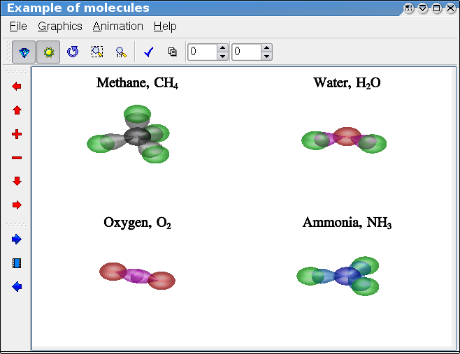
void setDraw (mglDraw *dr)Sets drawing functions from a class inherited from mglDraw.
void setDraw (int (*draw)(mglBase *gr, void *p), void *par=NULL)void setDraw (int (*draw)(mglGraph *gr))Sets the drawing function draw. There is support of a list of plots (frames). So as one can prepare a set of frames at first and redraw it fast later (but it requires more memory). Function should return positive number of frames for the list or zero if it will plot directly. Parameter par contains pointer to data for the plotting function draw.
void setGraph (HMGL gr)void setGraph (mglGraph *gr)Set pointer to external grapher (instead of built-in one). Note that QMathGL will automatically delete this object at destruction or at new setGraph() call.
HMGL getGraph ()Get pointer to grapher.
void setPopup (QMenu *p)Set popup menu pointer.
void setSize (int w, int h)Set widget/picture sizes
double getRatio ()Return aspect ratio of the picture.
int getPer ()Get perspective value in percents.
int getPhi ()Get Phi-angle value in degrees.
int getTet ()Get Theta-angle value in degrees.
bool getAlpha ()Get transparency state.
bool getLight ()Get lightning state.
bool getZoom ()Get mouse zooming state.
bool getRotate ()Get mouse rotation state.
QMathGL: void refresh ()Redraw saved bitmap without executing drawing function.
QMathGL: void update ()Update picture by executing drawing function.
QMathGL: void copy ()Copy graphics to clipboard.
QMathGL: void copyClickCoor ()Copy coordinates of click (as text).
QMathGL: void print ()Print current picture.
QMathGL: void stop ()Send signal to stop drawing.
QMathGL: void adjust ()Adjust image size to fit whole widget.
QMathGL: void nextSlide ()Show next slide.
QMathGL: void prevSlide ()Show previous slide.
QMathGL: void animation (bool st=true)Start/stop animation.
QMathGL: void setPer (int val)Set perspective value.
QMathGL: void setPhi (int val)Set Phi-angle value.
QMathGL: void setTet (int val)Set Theta-angle value.
QMathGL: void setAlpha (bool val)Switch on/off transparency.
QMathGL: void setLight (bool val)Switch on/off lightning.
QMathGL: void setGrid (bool val)Switch on/off drawing of grid for absolute coordinates.
QMathGL: void setZoom (bool val)Switch on/off mouse zooming.
QMathGL: void setRotate (bool val)Switch on/off mouse rotation.
QMathGL: void zoomIn ()Zoom in graphics.
QMathGL: void zoomOut ()Zoom out graphics.
QMathGL: void shiftLeft ()Shift graphics to left direction.
QMathGL: void shiftRight ()Shift graphics to right direction.
QMathGL: void shiftUp ()Shift graphics to up direction.
QMathGL: void shiftDown ()Shift graphics to down direction.
QMathGL: void restore ()Restore zoom and rotation to default values.
QMathGL: void exportPNG (QString fname="")Export current picture to PNG file.
QMathGL: void exportPNGs (QString fname="")Export current picture to PNG file (no transparency).
QMathGL: void exportJPG (QString fname="")Export current picture to JPEG file.
QMathGL: void exportBPS (QString fname="")Export current picture to bitmap EPS file.
QMathGL: void exportEPS (QString fname="")Export current picture to vector EPS file.
QMathGL: void exportSVG (QString fname="")Export current picture to SVG file.
QMathGL: void exportGIF (QString fname="")Export current picture to GIF file.
QMathGL: void exportTEX (QString fname="")Export current picture to LaTeX/Tikz file.
QMathGL: void exportTGA (QString fname="")Export current picture to TGA file.
QMathGL: void exportXYZ (QString fname="")Export current picture to XYZ/XYZL/XYZF file.
QMathGL: void exportOBJ (QString fname="")Export current picture to OBJ/MTL file.
QMathGL: void exportSTL (QString fname="")Export current picture to STL file.
QMathGL: void exportOFF (QString fname="")Export current picture to OFF file.
QMathGL: voidsetUsePrimitives (bool use)Enable using list of primitives for frames. This allows frames transformation/zoom but requires much more memory. Default value is true.
QMathGL: void setMGLFont (QString path)Restore (path="") or load font for graphics.
QMathGL: void about ()Show about information.
QMathGL: void aboutQt ()Show information about Qt version.
QMathGL: void phiChanged (int val)Phi angle changed (by mouse or by toolbar).
QMathGL: void tetChanged (int val)Tet angle changed (by mouse or by toolbar).
QMathGL: void perChanged (int val)Perspective changed (by mouse or by toolbar).
QMathGL: void alphaChanged (bool val)Transparency changed (by toolbar).
QMathGL: void lightChanged (bool val)Lighting changed (by toolbar).
QMathGL: void gridChanged (bool val)Grid drawing changed (by toolbar).
QMathGL: void zoomChanged (bool val)Zooming changed (by toolbar).
QMathGL: void rotateChanged (bool val)Rotation changed (by toolbar).
QMathGL: void mouseClick (mreal x, mreal y, mreal z)Mouse click take place at position {x,y,z}.
QMathGL: void frameChanged (int val)Need another frame to show.
QMathGL: void showWarn (QString warn)Need to show warning.
QMathGL: void posChanged (QString pos)Position of mouse click is changed.
QMathGL: void objChanged (int id)Object id is changed (due to mouse click).
QMathGL: void refreshData ()Data can be changed (drawing is finished).
QString appNameApplication name for message boxes.
bool autoResizeAllow auto resizing (default is false).
Previous: QMathGL class, Up: Widget classes [Contents][Index]
Class is WX widget which display MathGL graphics. It is defined in #include <mgl2/wx.h>.
void SetDraw (mglDraw *dr)Sets drawing functions from a class inherited from mglDraw.
void SetDraw (int (*draw)(mglBase *gr, void *p), void *par=NULL)void SetDraw (int (*draw)(mglGraph *gr))Sets the drawing function draw. There is support of a list of plots (frames). So as one can prepare a set of frames at first and redraw it fast later (but it requires more memory). Function should return positive number of frames for the list or zero if it will plot directly. Parameter par contains pointer to data for the plotting function draw.
void SetGraph (HMGL gr)void SetGraph (mglGraph *gr)Set pointer to external grapher (instead of built-in one). Note that wxMathGL will automatically delete this object at destruction or at new setGraph() call.
HMGL GetGraph ()Get pointer to grapher.
void SetPopup (wxMenu *p)Set popup menu pointer.
void SetSize (int w, int h)Set widget/picture sizes
double GetRatio ()Return aspect ratio of the picture.
int GetPer ()Get perspective value in percents.
int GetPhi ()Get Phi-angle value in degrees.
int GetTet ()Get Theta-angle value in degrees.
bool GetAlpha ()Get transparency state.
bool GetLight ()Get lightning state.
bool GetZoom ()Get mouse zooming state.
bool GetRotate ()Get mouse rotation state.
void Repaint ()Redraw saved bitmap without executing drawing function.
void Update ()Update picture by executing drawing function.
void Copy ()Copy graphics to clipboard.
void Print ()Print current picture.
void Adjust ()Adjust image size to fit whole widget.
void NextSlide ()Show next slide.
void PrevSlide ()Show previous slide.
void Animation (bool st=true)Start/stop animation.
void SetPer (int val)Set perspective value.
void SetPhi (int val)Set Phi-angle value.
void SetTet (int val)Set Theta-angle value.
void SetAlpha (bool val)Switch on/off transparency.
void SetLight (bool val)Switch on/off lightning.
void SetZoom (bool val)Switch on/off mouse zooming.
void SetRotate (bool val)Switch on/off mouse rotation.
void ZoomIn ()Zoom in graphics.
void ZoomOut ()Zoom out graphics.
void ShiftLeft ()Shift graphics to left direction.
void ShiftRight ()Shift graphics to right direction.
void ShiftUp ()Shift graphics to up direction.
void ShiftDown ()Shift graphics to down direction.
void Restore ()Restore zoom and rotation to default values.
void About ()Show about information.
void ExportPNG (QString fname="")Export current picture to PNG file.
void ExportPNGs (QString fname="")Export current picture to PNG file (no transparency).
void ExportJPG (QString fname="")Export current picture to JPEG file.
void ExportBPS (QString fname="")Export current picture to bitmap EPS file.
void ExportEPS (QString fname="")Export current picture to vector EPS file.
void ExportSVG (QString fname="")Export current picture to SVG file.
Next: MGL scripts, Previous: Widget classes, Up: Top [Contents][Index]
This chapter describe classes mglData and mglDataC for working with data arrays of real and complex numbers. Both classes are derived from abstract class mglDataA, and can be used as arguments of any plotting functions (see MathGL core). These classes are defined in #include <mgl2/data.h> and #include <mgl2/datac.h> correspondingly. The classes have mostly the same set of functions for easy and safe allocation, resizing, loading, saving, modifying of data arrays. Also it can numerically differentiate and integrate data, interpolate, fill data by formula and so on. Classes support data with dimensions up to 3 (like function of 3 variables – x,y,z). The internal representation of numbers is mreal (or dual=std::complex<mreal> for mglDataC), which can be configured as float or double by selecting option --enable-double at the MathGL configuring (see Installation). Float type have smaller size in memory and usually it has enough precision in plotting purposes. However, double type provide high accuracy what can be important for time-axis, for example. Data arrays are denoted by Small Caps (like DAT) if it can be (re-)created by MGL commands.
Next: Data constructor, Up: Data processing [Contents][Index]
mreal * adual * aData array itself. The flat data representation is used. For example, matrix [nx x ny] is presented as flat (1d-) array with length nx*ny. The element with indexes {i, j, k} is a[i+nx*j+nx*ny*k] (indexes are zero based).
long nxlong nxNumber of points in 1st dimensions (’x’ dimension).
long nylong nyNumber of points in 2nd dimensions (’y’ dimension).
long nzlong nzNumber of points in 3d dimensions (’z’ dimension).
std::string idstd::string idNames of column (or slice if nz>1) – one character per column.
bool linkbool linkFlag to use external data, i.e. don’t delete it.
std::wstring sName of data. It is used in parsing of MGL scripts.
bool tempFlag of temporary variable, which should be deleted.
void (*)(void *) funcPointer to callback function which will be called at destroying.
void * oPointer to object for callback function.
mglData: mreal GetVal (long i)mglDataC: mreal GetVal (long i)mglData: void SetVal (mreal val, long i)mglDataC: void SetVal (mreal val, long i)Gets or sets the value in by "flat" index i without border checking. Index i should be in range [0, nx*ny*nz-1].
mglDataA: long GetNx ()mglDataA: long GetNy ()mglDataA: long GetNz ()long mgl_data_get_nx (HCDT dat)long mgl_data_get_ny (HCDT dat)long mgl_data_get_nz (HCDT dat)Gets the x-, y-, z-size of the data.
mreal mgl_data_get_value (HCDT dat, int i, int j, int k)dual mgl_datac_get_value (HCDT dat, int i, int j, int k)mreal * mgl_data_value (HMDT dat, int i, int j, int k)dual * mgl_datac_value (HADT dat, int i, int j, int k)void mgl_data_set_value (HMDT dat, mreal v, int i, int j, int k)void mgl_datac_set_value (HADT dat, dual v, int i, int j, int k)Gets or sets the value in specified cell of the data with border checking.
const mreal * mgl_data_data (HCDT dat)const dual * mgl_datac_data (HCDT dat)Returns pointer to internal data array.
void mgl_data_set_func (mglDataA *dat, void (*func)(void *), void *par)Set pointer to callback function which will be called at destroying.
void mgl_data_set_name (mglDataA *dat, const char *name)void mgl_data_set_name_w (mglDataA *dat, const wchar_t *name)Set name of data, which used in parsing of MGL scripts.
Next: Data resizing, Previous: Public variables, Up: Data processing [Contents][Index]
nx=1 'eq']nx ny ['eq']nx ny nz ['eq']mglData: mglData (int mx=1, int my=1, int mz=1)mglDataC: mglDataC (int mx=1, int my=1, int mz=1)HMDT mgl_create_data ()HMDT mgl_create_data_size (int mx, int my, int mz)HADT mgl_create_datac ()HADT mgl_create_datac_size (int mx, int my, int mz)Default constructor. Allocates the memory for data array and initializes it by zero. If string eq is specified then data will be filled by corresponding formula as in fill.
valmglData: mglData (const mglDataA &dat2)mglData: mglData (const mglDataA *dat2)mglData: mglData (int size, const float *dat2)mglData: mglData (int size, int cols, const float *dat2)mglData: mglData (int size, const double *dat2)mglData: mglData (int size, int cols, const double *dat2)mglData: mglData (const double *dat2, int size)mglData: mglData (const double *dat2, int size, int cols)mglDataC: mglDataC (const mglDataA &dat2)mglDataC: mglDataC (const mglDataA *dat2)mglDataC: mglDataC (int size, const float *dat2)mglDataC: mglDataC (int size, int cols, const float *dat2)mglDataC: mglDataC (int size, const double *dat2)mglDataC: mglDataC (int size, int cols, const double *dat2)mglDataC: mglDataC (int size, const dual *dat2)mglDataC: mglDataC (int size, int cols, const dual *dat2)Copy constructor. Allocates the memory for data array and copy values from other array. At this, if parameter eq or val is specified then the data will be modified by corresponding formula similarly to fill.
Allocates the memory for data array and copy real and imaginary values from complex array dat2.
Allocates the memory for data array and copy values from other array specified by its name, which can be "invalid" for MGL names (like one read from HDF5 files).
mglData: mglData (const char *fname)mglDataC: mglDataC (const char *fname)HMDT mgl_create_data_file (const char *fname)HADT mgl_create_datac_file (const char *fname)Reads data from tab-separated text file with auto determining sizes of the data.
mglData: ~mglData ()void mgl_delete_data (HMDT dat)mglDataC: ~mglDataC ()void mgl_delete_datac (HADT dat)Deletes the data array from memory.
Next: Data filling, Previous: Data constructor, Up: Data processing [Contents][Index]
nx=1 ny=1 nz=1]mglData: void Create (int mx, int my=1, int mz=1)mglDataC: void Create (int mx, int my=1, int mz=1)void mgl_data_create (HMDT dat, int mx, int my, int mz)void mgl_datac_create (HADT dat, int mx, int my, int mz)Creates or recreates the array with specified size and fills it by zero. This function does nothing if one of parameters mx, my, mz is zero or negative.
mx [my=0 mz=0]mglData: void Rearrange (int mx, int my=0, int mz=0)mglDataC: void Rearrange (int mx, int my=0, int mz=0)void mgl_data_rearrange (HMDT dat, int mx, int my, int mz)void mgl_datac_rearrange (HADT dat, int mx, int my, int mz)Rearrange dimensions without changing data array so that resulting sizes should be mx*my*mz < nx*ny*nz. If some of parameter my or mz are zero then it will be selected to optimal fill of data array. For example, if my=0 then it will be change to my=nx*ny*nz/mx and mz=1.
mglData: void Transpose (const char *dim="yx")mglDataC: void Transpose (const char *dim="yx")void mgl_data_transpose (HMDT dat, const char *dim)void mgl_datac_transpose (HADT dat, const char *dim)Transposes (shift order of) dimensions of the data. New order of dimensions is specified in string dim. This function can be useful also after reading of one-dimensional data.
n1 [n2=0]mglData: void Extend (int n1, int n2=0)mglDataC: void Extend (int n1, int n2=0)void mgl_data_extend (HMDT dat, int n1, int n2)void mgl_datac_extend (HADT dat, int n1, int n2)Increase the dimensions of the data by inserting new (|n1|+1)-th slices after (for n1>0) or before (for n1<0) of existed one. It is possible to insert 2 dimensions simultaneously for 1d data by using parameter n2. Data to new slices is copy from existed one. For example, for n1>0 new array will be a_ij^new = a_i^old where j=0...n1. Correspondingly, for n1<0 new array will be a_ij^new = a_j^old where i=0...|n1|.
rx [ry=1 rz=1 sm=off]mglData: void Squeeze (int rx, int ry=1, int rz=1, bool smooth=false)mglDataC: void Squeeze (int rx, int ry=1, int rz=1, bool smooth=false)void mgl_data_squeeze (HMDT dat, int rx, int ry, int rz, int smooth)void mgl_datac_squeeze (HADT dat, int rx, int ry, int rz, int smooth)Reduces the data size by excluding data elements which indexes are not divisible by rx, ry, rz correspondingly. Parameter smooth set to use smoothing (i.e. out[i]=\sum_{j=i,i+r} a[j]/r) or not (i.e. out[i]=a[j*r]).
n1 n2 'dir'mglData: void Crop (int n1, int n2, char dir='x')mglDataC: void Crop (int n1, int n2, char dir='x')void mgl_data_crop (HMDT dat, int n1, int n2, char dir)void mgl_datac_crop (HADT dat, int n1, int n2, char dir)Cuts off edges of the data i<n1 and i>n2 if n2>0 or i>n[xyz]-n2 if n2<=0 along direction dir.
mglData: void Crop (const char *how="235x")mglDataC: void Crop (const char *how="235x")void mgl_data_crop_opt (HMDT dat, const char *how)void mgl_datac_crop_opt (HADT dat, const char *how)Cuts off far edge of the data to be more optimal for fast Fourier transform. The resulting size will be the closest value of 2^n*3^m*5^l to the original one. The string how may contain: ‘x’, ‘y’, ‘z’ for directions, and ‘2’, ‘3’, ‘5’ for using corresponding bases.
[pos=off num=0]mglData: void Insert (char dir, int pos=0, int num=1)mglDataC: void Insert (char dir, int pos=0, int num=1)void mgl_data_insert (HMDT dat, char dir, int pos, char num)void mgl_datac_insert (HADT dat, char dir, int pos, char num)Insert num slices along dir-direction at position pos and fill it by zeros.
[pos=off num=0]mglData: void Delete (char dir, int pos=0, int num=1)mglDataC: void Delete (char dir, int pos=0, int num=1)void mgl_data_delete (HMDT dat, char dir, int pos, char num)void mgl_datac_delete (HADT dat, char dir, int pos, char num)Delete num slices along dir-direction at position pos.
Deletes the whole data array.
idx [idy=-1]mglData: void Sort (lond idx, long idy=-1)void mgl_data_sort (HMDT dat, lond idx, long idy)Sort data rows (or slices in 3D case) by values of specified column idx (or cell {idx,idy} for 3D case). Note, this function is not thread safe!
idxmglData: void Clean (lond idx)void mgl_data_clean (HMDT dat, lond idx)Delete rows which values are equal to next row for given column idx.
mglData: void Join (const mglDataA &vdat)mglDataC: void Join (const mglDataA &vdat)void mgl_data_join (HMDT dat, HCDT vdat)void mgl_datac_join (HADT dat, HCDT vdat)Join data cells from vdat to dat. At this, function increase dat sizes according following: z-size for data arrays arrays with equal x-,y-sizes; or y-size for data arrays with equal x-sizes; or x-size otherwise.
Next: File I/O, Previous: Data resizing, Up: Data processing [Contents][Index]
v1 ...Creates new variable with name dat and fills it by numeric values of command arguments v1 .... Command can create one-dimensional and two-dimensional arrays with arbitrary values. For creating 2d array the user should use delimiter ‘|’ which means that the following values lie in next row. Array sizes are [maximal of row sizes * number of rows]. For example, command list 1 | 2 3 creates the array [1 0; 2 3]. Note, that the maximal number of arguments is 1000.
Creates new variable with name dat and fills it by data values of arrays of command arguments d1 .... Command can create two-dimensional or three-dimensional (if arrays in arguments are 2d arrays) arrays with arbitrary values. Minor dimensions of all arrays in arguments should be equal to dimensions of first array d1. In the opposite case the argument will be ignored. Note, that the maximal number of arguments is 1000.
mglData: void Set (const float *A, int NX, int NY=1, int NZ=1)mglData: void Set (const double *A, int NX, int NY=1, int NZ=1)void mgl_data_set_float (HMDT dat, const mreal *A, int NX, int NY, int NZ)void mgl_data_set_double (HMDT dat, const double *A, int NX, int NY, int NZ)mglDataC: void Set (const float *A, int NX, int NY=1, int NZ=1)mglDataC: void Set (const double *A, int NX, int NY=1, int NZ=1)mglDataC: void Set (const dual *A, int NX, int NY=1, int NZ=1)void mgl_datac_set_float (HADT dat, const mreal *A, int NX, int NY, int NZ)void mgl_datac_set_double (HADT dat, const double *A, int NX, int NY, int NZ)void mgl_datac_set_complex (HADT dat, const dual *A, int NX, int NY, int NZ)Allocates memory and copies the data from the flat float* or double* array.
mglData: void Set (const float **A, int N1, int N2)mglData: void Set (const double **A, int N1, int N2)void mgl_data_set_mreal2 (HMDT dat, const mreal **A, int N1, int N2)void mgl_data_set_double2 (HMDT dat, const double **A, int N1, int N2)Allocates memory and copies the data from the float** or double** array with dimensions N1, N2, i.e. from array defined as mreal a[N1][N2];.
mglData: void Set (const float ***A, int N1, int N2)mglData: void Set (const double ***A, int N1, int N2)void mgl_data_set_mreal3 (HMDT dat, const mreal ***A, int N1, int N2)void mgl_data_set_double3 (HMDT dat, const double ***A, int N1, int N2)Allocates memory and copies the data from the float*** or double*** array with dimensions N1, N2, N3, i.e. from array defined as mreal a[N1][N2][N3];.
mglData: void Set (gsl_vector *v)mglDataC: void Set (gsl_vector *v)void mgl_data_set_vector (HMDT dat, gsl_vector *v)void mgl_datac_set_vector (HADT dat, gsl_vector *v)Allocates memory and copies the data from the gsl_vector * structure.
mglData: void Set (gsl_matrix *m)mglDataC: void Set (gsl_matrix *m)void mgl_data_set_matrix (HMDT dat, gsl_matrix *m)void mgl_datac_set_matrix (HADT dat, gsl_matrix *m)Allocates memory and copies the data from the gsl_matrix * structure.
mglData: void Set (const mglDataA &from)mglData: void Set (HCDT from)void mgl_data_set (HMDT dat, HCDT from)mglDataC: void Set (const mglDataA &from)mglDataC: void Set (HCDT from)void mgl_datac_set (HADT dat, HCDT from)Copies the data from mglData (or mglDataA) instance from.
mglDataC: void Set (const mglDataA &re, const mglDataA &im)mglDataC: void Set (HCDT re, HCDT im)mglDataC: void SetAmpl (HCDT ampl, const mglDataA &phase)void mgl_datac_set_ri (HADT dat, HCDT re, HCDT im)void mgl_datac_set_ap (HADT dat, HCDT ampl, HCDT phase)Copies the data from mglData instances for real and imaginary parts of complex data arrays.
mglData: void Set (const std::vector<int> &d)mglDataC: void Set (const std::vector<int> &d)mglData: void Set (const std::vector<float> &d)mglDataC: void Set (const std::vector<float> &d)mglData: void Set (const std::vector<double> &d)mglDataC: void Set (const std::vector<double> &d)mglDataC: void Set (const std::vector<dual> &d)Allocates memory and copies the data from the std::vector<T> array.
mglData: void Set (const char *str, int NX, int NY=1, int NZ=1)void mgl_data_set_values (const char *str, int NX, int NY, int NZ)mglDataC: void Set (const char *str, int NX, int NY=1, int NZ=1)void mgl_datac_set_values (const char *str, int NX, int NY, int NZ)Allocates memory and scanf the data from the string.
mglData: void SetList (long n, ...)Allocate memory and set data from variable argument list of double values. Note, you need to specify decimal point ‘.’ for integer values! For example, the code SetList(2,0.,1.); is correct, but the code SetList(2,0,1); is incorrect.
mglData: void Set (const arma::vec &d)mglData: void Set (const arma::mat &d)mglData: void Set (const arma::cube &d)mglDataC: void Set (const arma::vec &d)mglDataC: void Set (const arma::cx_vec &d)mglDataC: void Set (const arma::mat &d)mglDataC: void Set (const arma::cx_mat &d)mglDataC: void Set (const arma::cube &d)mglDataC: void Set (const arma::cx_cube &d)Allocates memory and copies the data from the Armadillo structures.
mglData: arma::mat arma_mat (long k=0)mglData: arma::cube arma_cube ()mglData: arma::cx_mat arma_mat (long k=0)mglData: arma::cx_cube arma_cube ()Return data in Armadillo format.
mglData: void Link (mglData &from)mglData: void Link (mreal *A, int NX, int NY=1, int NZ=1)void mgl_data_link (HMDT dat, mreal *A, int NX, int NY, int NZ)mglDataC: void Link (mglDataC &from)mglDataC: void Link (dual *A, int NX, int NY=1, int NZ=1)void mgl_datac_link (HADT dat, dual *A, int NX, int NY, int NZ)Links external data array, i.e. don’t delete this array at exit.
num v1 [v2=nan]Creates new variable with name dat for one-dimensional array of size num. Array elements are equidistantly distributed in range [v1, v2]. If v2=nan then v2=v1 is used.
mglData: void Fill (mreal v1, mreal v2, char dir='x')mglDataC: void Fill (dual v1, dual v2, char dir='x')void mgl_data_fill (HMDT dat, mreal v1, mreal v2, char dir)void mgl_datac_fill (HADT dat, dual v1, dual v2, char dir)Equidistantly fills the data values to range [v1, v2] in direction dir={‘x’,‘y’,‘z’}.
mglData: void Fill (HMGL gr, const char *eq, const char *opt="")mglData: void Fill (HMGL gr, const char *eq, const mglDataA &vdat, const char *opt="")mglData: void Fill (HMGL gr, const char *eq, const mglDataA &vdat, const mglDataA &wdat, const char *opt="")mglDataC: void Fill (HMGL gr, const char *eq, const char *opt="")mglDataC: void Fill (HMGL gr, const char *eq, const mglDataA &vdat, const char *opt="")mglDataC: void Fill (HMGL gr, const char *eq, const mglDataA &vdat, const mglDataA &wdat, const char *opt="")void mgl_data_fill_eq (HMGL gr, HMDT dat, const char *eq, HCDT vdat, HCDT wdat, const char *opt)void mgl_datac_fill_eq (HMGL gr, HADT dat, const char *eq, HCDT vdat, HCDT wdat, const char *opt)Fills the value of array according to the formula in string eq. Formula is an arbitrary expression depending on variables ‘x’, ‘y’, ‘z’, ‘u’, ‘v’, ‘w’. Coordinates ‘x’, ‘y’, ‘z’ are supposed to be normalized in axis range of canvas gr (in difference from Modify functions). Variables ‘i’, ‘j’, ‘k’ denote corresponding index. At this, zero value is used for variables if corresponding dimension is absent in the data. Variable ‘u’ is the original value of the array. Variables ‘v’ and ‘w’ are values of vdat, wdat which can be NULL (i.e. can be omitted).
dim=0]mglData: void Modify (const char *eq, int dim=0)mglData: void Modify (const char *eq, const mglDataA &v)mglData: void Modify (const char *eq, const mglDataA &v, const mglDataA &w)mglDataC: void Modify (const char *eq, int dim=0)mglDataC: void Modify (const char *eq, const mglDataA &v)mglDataC: void Modify (const char *eq, const mglDataA &v, const mglDataA &w)void mgl_data_modify (HMDT dat, const char *eq, int dim)void mgl_data_modify_vw (HMDT dat, const char *eq, HCDT v, HCDT w)void mgl_datac_modify (HADT dat, const char *eq, int dim)void mgl_datac_modify_vw (HADT dat, const char *eq, HCDT v, HCDT w)The same as previous ones but coordinates ‘x’, ‘y’, ‘z’ are supposed to be normalized in range [0,1]. Variables ‘i’, ‘j’, ‘k’ denote corresponding index. At this, zero value is used for variables if corresponding dimension is absent in the data. If dim>0 is specified then modification will be fulfilled only for slices >=dim.
mglData: void FillSample (const char *how)void mgl_data_fill_sample (HMDT a, const char *how)Fills data by ’x’ or ’k’ samples for Hankel (’h’) or Fourier (’f’) transform.
mglData: mglData Grid (HMGL gr, const mglDataA &x, const mglDataA &y, const mglDataA &z, const char *opt="")mglData: mglData Grid (const mglDataA &x, const mglDataA &y, const mglDataA &z, mglPoint p1, mglPoint p2)void mgl_data_grid (HMGL gr, HMDT u, HCDT x, HCDT y, HCDT z, const char *opt)void mgl_data_grid_xy (HMDT u, HCDT x, HCDT y, HCDT z, mreal x1, mreal x2, mreal y1, mreal y2)Fills the value of array according to the linear interpolation of triangulated surface assuming x-,y-coordinates equidistantly distributed in axis range (or in range [x1,x2]*[y1,y2]). Triangulated surface is found for arbitrary placed points ‘x’, ‘y’, ‘z’. NAN value is used for grid points placed outside of triangulated surface. See Making regular data, for sample code and picture.
val [i=all j=all k=all]mglData: void Put (mreal val, int i=-1, int j=-1, int k=-1)mglDataC: void Put (dual val, int i=-1, int j=-1, int k=-1)void mgl_data_put_val (HMDT a, mreal val, int i, int j, int k)void mgl_datac_put_val (HADT a, dual val, int i, int j, int k)Sets value(s) of array a[i, j, k] = val. Negative indexes i, j, k=-1 set the value val to whole range in corresponding direction(s). For example, Put(val,-1,0,-1); sets a[i,0,j]=val for i=0...(nx-1), j=0...(nz-1).
i=all j=all k=all]mglData: void Put (const mglDataA &v, int i=-1, int j=-1, int k=-1)mglDataC: void Put (const mglDataA &v, int i=-1, int j=-1, int k=-1)void mgl_data_put_dat (HMDT a, HCDT v, int i, int j, int k)void mgl_datac_put_dat (HADT a, HCDT v, int i, int j, int k)Copies value(s) from array v to the range of original array. Negative indexes i, j, k=-1 set the range in corresponding direction(s). At this minor dimensions of array v should be large than corresponding dimensions of this array. For example, Put(v,-1,0,-1); sets a[i,0,j]=v.ny>nz ? v[i,j] : v[i], where i=0...(nx-1), j=0...(nz-1) and condition v.nx>=nx is true.
mglData: void Refill (const mglDataA &x, const mglDataA &v, mreal x1, mreal x2, long sl=-1)mglData: void Refill (const mglDataA &x, const mglDataA &v, mglPoint p1, mglPoint p2, long sl=-1)mglData: void Refill (const mglDataA &x, const mglDataA &y, const mglDataA &v, mglPoint p1, mglPoint p2, long sl=-1)mglData: void Refill (const mglDataA &x, const mglDataA &y, const mglDataA &z, const mglDataA &v, mglPoint p1, mglPoint p2)mglData: void Refill (HMGL gr, const mglDataA &x, const mglDataA &v, long sl=-1, const char *opt="")mglData: void Refill (HMGL gr, const mglDataA &x, const mglDataA &y, const mglDataA &v, long sl=-1, const char *opt="")mglData: void Refill (HMGL gr, const mglDataA &x, const mglDataA &y, const mglDataA &z, const mglDataA &v, const char *opt="")void mgl_data_refill_x (HMDT a, HCDT x, HCDT v, mreal x1, mreal x2, long sl)void mgl_data_refill_xy (HMDT a, HCDT x, HCDT y, HCDT v, mreal x1, mreal x2, mreal y1, mreal y2, long sl)void mgl_data_refill_xyz (HMDT a, HCDT x, HCDT y, HCDT z, HCDT v, mreal x1, mreal x2, mreal y1, mreal y2, mreal z1, mreal z2)void mgl_data_refill_gr (HMGL gr, HMDT a, HCDT x, HCDT y, HCDT z, HCDT v, long sl, const char *opt)Fills by interpolated values of array v at the point {x, y, z}={X[i], Y[j], Z[k]} (or {x, y, z}={X[i,j,k], Y[i,j,k], Z[i,j,k]} if x, y, z are not 1d arrays), where X,Y,Z are equidistantly distributed in range [x1,x2]*[y1,y2]*[z1,z2] and have the same sizes as this array. If parameter sl is 0 or positive then changes will be applied only for slice sl.
mglData: void RefillGS (const mglDataA &x, const mglDataA &v, mreal x1, mreal x2, long sl=-1)void mgl_data_refill_gs (HMDT a, HCDT x, HCDT v, mreal x1, mreal x2, long sl)Fills by global cubic spline values of array v at the point x=X[i], where X are equidistantly distributed in range [x1,x2] and have the same sizes as this array. If parameter sl is 0 or positive then changes will be applied only for slice sl.
mglData: void SetColumnId (const char *ids)mglDataC: void SetColumnId (const char *ids)void mgl_data_set_id (HMDT a, const char *ids)void mgl_datac_set_id (HADT a, const char *ids)Sets the symbol ids for data columns. The string should contain one symbol ’a’...’z’ per column. These ids are used in column.
p=0.5]mglData: void RndBernoulli (mreal p=0.5)void mgl_data_rnd_bernoulli (HMDT dat, mreal p)mreal mgl_rnd_bernoulli (mreal p)Fills data by random numbers of Bernoulli distribution with probability p.
n [p=0.5]mglData: void RndBinomial (long n, mreal p=0.5)void mgl_data_rnd_binomial (HMDT dat, long n, mreal p)mreal mgl_rnd_binomial (long n, mreal p)Fills by random numbers according to binomial distribution in n coin flips with probability p.
y1 y2 sigma hmglData: void RndBrownian (mreal y1, mreal y2, mreal sigma, mreal h)void mgl_data_rnd_brownian (HMDT dat, mreal y1, mreal y2, mreal sigma, mreal h)Fills by fractional brownian motion.
mglData: void RndDiscrete (const mglDataA &vdat)void mgl_data_rnd_discrete (HMDT dat, HCDT vdat)mreal mgl_rnd_discrete (HCDT vdat)Fills by random numbers according to discrete distribution.
p]mglData: void RndExponential (mreal p)void mgl_data_rnd_exponential (HMDT dat, mreal p)mreal mgl_rnd_exponential (mreal p)Fills by random numbers according to exponential distribution with scale p.
mu=0 sigma=1]mglData: void RndGaussian (mreal mu=0, mreal sigma=1)void mgl_data_rnd_gaussian (HMDT dat, mreal mu, mreal sigma)mreal mgl_rnd_gaussian (mreal mu, mreal sigma)Fills by random numbers according to Gaussian distribution with average mu and scale sigma.
mglData: void RndShuffle (char dir='a')void mgl_data_rnd_shuffle (HMDT dat, char dir)Shuffle data cells (for dir=‘a’) or slices (for dir=‘xyz’).
lo himglData: void RndUniform (mreal lo, mreal hi)void mgl_data_rnd_uniform (HMDT dat, mreal lo, mreal hi)mreal mgl_rnd_uniform (mreal lo, mreal hi)Fills by random numbers uniformly chosen in (lo,hi).
lo himglData: void RndInteger (long lo, long hi)void mgl_data_rnd_integer (HMDT dat, long lo, mreal hi)long mgl_rnd_integer (long lo, long hi)Fills by random integers uniformly chosen in [lo,hi).
Next: Make another data, Previous: Data filling, Up: Data processing [Contents][Index]
mglData: bool Read (const char *fname)mglDataC: bool Read (const char *fname)int mgl_data_read (HMDT dat, const char *fname)int mgl_datac_read (HADT dat, const char *fname)Reads data from tab-separated text file with auto determining sizes of the data. Double newline means the beginning of new z-slice.
mx [my=1 mz=1]mx [my=1 mz=1]mglData: bool Read (const char *fname, int mx, int my=1, int mz=1)mglDataC: bool Read (const char *fname, int mx, int my=1, int mz=1)int mgl_data_read_dim (HMDT dat, const char *fname, int mx, int my, int mz)int mgl_datac_read_dim (HADT dat, const char *fname, int mx, int my, int mz)Reads data from text file with specified data sizes. This function does nothing if one of parameters mx, my or mz is zero or negative.
dim=2]mglData: bool ReadMat (const char *fname, int dim=2)mglDataC: bool ReadMat (const char *fname, int dim=2)int mgl_data_read_mat (HMDT dat, const char *fname, int dim)int mgl_datac_read_mat (HADT dat, const char *fname, int dim)Read data from text file with size specified at beginning of the file by first dim numbers. At this, variable dim set data dimensions.
v1 v2 [dv=1 slice=off]mglData: void ReadRange (const char *templ, mreal from, mreal to, mreal step=1, bool as_slice=false)mglDataC: void ReadRange (const char *templ, mreal from, mreal to, mreal step=1, bool as_slice=false)int mgl_data_read_range (HMDT dat, const char *templ, mreal from, mreal to, mreal step, int as_slice)int mgl_datac_read_range (HADT dat, const char *templ, mreal from, mreal to, mreal step, int as_slice)Join data arrays from several text files. The file names are determined by function call sprintf(fname,templ,val);, where val changes from from to to with step step. The data load one-by-one in the same slice if as_slice=false or as slice-by-slice if as_slice=true.
[slice=off]mglData: void ReadAll (const char *templ, bool as_slice=false)mglDataC: void ReadAll (const char *templ, bool as_slice=false)int mgl_data_read_all (HMDT dat, const char *templ, int as_slice)int mgl_datac_read_all (HADT dat, const char *templ, int as_slice)Join data arrays from several text files which filenames satisfied the template templ (for example, templ="t_*.dat"). The data load one-by-one in the same slice if as_slice=false or as slice-by-slice if as_slice=true.
mglData: bool ScanFile (const char *fname, const char *templ)int mgl_data_scan_file (HMDT dat, const char *fname, const char *templ)Read file fname line-by-line and scan each line for numbers according the template templ. The numbers denoted as ‘%g’ in the template. See Saving and scanning file, for sample code and picture.
mglDataA: void Save (const char *fname, int ns=-1) constvoid mgl_data_save (HCDT dat, const char *fname, int ns)void mgl_datac_save (HCDT dat, const char *fname, int ns)Saves the whole data array (for ns=-1) or only ns-th slice to the text file fname.
val dat 'fname'Saves the value val to the text file fname.
Saves the string str to the text file fname. For parameter mode=‘a’ will append string to the file (default); for mode=‘w’ will overwrite the file. See Saving and scanning file, for sample code and picture.
mglData: void ReadHDF (const char *fname, const char *dname)mglDataC: void ReadHDF (const char *fname, const char *dname)void mgl_data_read_hdf (HMDT dat, const char *fname, const char *dname)void mgl_datac_read_hdf (HADT dat, const char *fname, const char *dname)Reads data array named dname from HDF5 or HDF4 file. This function does nothing if HDF5|HDF4 was disabled during library compilation.
rewrite=off]mglDataA: void SaveHDF (const char *fname, const char *dname, bool rewrite=false) constvoid mgl_data_save_hdf (HCDT dat, const char *fname, const char *dname, int rewrite)void mgl_datac_save_hdf (HCDT dat, const char *fname, const char *dname, int rewrite)Saves data array named dname to HDF5 file. This function does nothing if HDF5 was disabled during library compilation.
val 'fname' 'dname' [rewrite=off]void mgl_real_save_hdf (real val, const char *fname, const char *dname, int rewrite)void mgl_dual_save_hdf (dual val, const char *fname, const char *dname, int rewrite)void mgl_int_save_hdf (long val, const char *fname, const char *dname, int rewrite)Saves value val named dname to HDF5 file. This function does nothing if HDF5 was disabled during library compilation.
mglDataA: int DatasHDF (const char *fname, char *buf, long size) staticint mgl_datas_hdf (const char *fname, char *buf, long size)Put data names from HDF5 file fname into buf as ’\t’ separated fields. In MGL version the list of data names will be printed as message. This function does nothing if HDF5 was disabled during library compilation.
mglParse: void OpenHDF (const char *fname)void mgl_parser_openhdf (HMPR pr, const char *fname)Reads all data array from HDF5 file fname and create MGL variables with names of data names in HDF file. Complex variables will be created if data name starts with ‘!’.
const char * const * mgl_datas_hdf_str (HMPR pr, const char *fname)Put HDF data names as list of strings (last one is ""). The result is valid untill next call of the function.
v1=0 v2=1]mglData: void Import (const char *fname, const char *scheme, mreal v1=0, mreal v2=1)void mgl_data_import (HMDT dat, const char *fname, const char *scheme, mreal v1, mreal v2)Reads data from bitmap file (now support only PNG format). The RGB values of bitmap pixels are transformed to mreal values in range [v1, v2] using color scheme scheme (see Color scheme).
v1=0 v2=0]mglDataA: void Export (const char *fname, const char *scheme, mreal v1=0, mreal v2=0, int ns=-1) constvoid mgl_data_export (HMDT dat, const char *fname, const char *scheme, mreal v1, mreal v2, int ns) constSaves data matrix (or ns-th slice for 3d data) to bitmap file (now support only PNG format). The data values are transformed from range [v1, v2] to RGB pixels of bitmap using color scheme scheme (see Color scheme). If v1>=v2 then the values of v1, v2 are automatically determined as minimal and maximal value of the data array.
typemglData: bool ReadBin (const char *fname, int type)int mgl_data_read_bin (HMDT dat, const char *fname, int type)Reads data from binary file. Parameter type determine the number format: 0 - double, 1 - float, 2 - long double, 3 - long int, 4 - int, 5 - short int, 6 - char. NOTE: this function may not correctly read binary files written in different CPU kind! It is better to use HDF files, see readhdf.
Next: Data changing, Previous: File I/O, Up: Data processing [Contents][Index]
xx [yy=all zz=all]mglData: mglData SubData (mreal xx, mreal yy=-1, mreal zz=-1) constmglDataC: mglData SubData (mreal xx, mreal yy=-1, mreal zz=-1) constHMDT mgl_data_subdata (HCDT dat, mreal xx, mreal yy, mreal zz)Extracts sub-array data from the original data array keeping fixed positive index. For example SubData(-1,2) extracts 3d row (indexes are zero based), SubData(4,-1) extracts 5th column, SubData(-1,-1,3) extracts 4th slice and so on. If argument(s) are non-integer then linear interpolation between slices is used. In MGL version this command usually is used as inline one dat(xx,yy,zz). Function return NULL or create empty data if data cannot be created for given arguments.
mglData: mglData SubData (const mglDataA &xx, const mglDataA &yy, const mglDataA &zz) constmglDataC: mglData SubData (const mglDataA &xx, const mglDataA &yy, const mglDataA &zz) constmglData: mglData SubData (const mglDataA &xx, const mglDataA &yy) constmglDataC: mglData SubData (const mglDataA &xx, const mglDataA &yy) constmglData: mglData SubData (const mglDataA &xx) constmglDataC: mglData SubData (const mglDataA &xx) constHMDT mgl_data_subdata_ext (HCDT dat, HCDT xx, HCDT yy, HCDT zz)HADT mgl_datac_subdata_ext (HCDT dat, HCDT xx, HCDT yy, HCDT zz)Extracts sub-array data from the original data array for indexes specified by arrays xx, yy, zz (indirect access). This function work like previous one for 1D arguments or numbers, and resulting array dimensions are equal dimensions of 1D arrays for corresponding direction. For 2D and 3D arrays in arguments, the resulting array have the same dimensions as input arrays. The dimensions of all argument must be the same (or to be scalar 1*1*1) if they are 2D or 3D arrays. In MGL version this command usually is used as inline one dat(xx,yy,zz). Function return NULL or create empty data if data cannot be created for given arguments. In C function some of xx, yy, zz can be NULL.
mglData: mglData Column (const char *eq) constmglDataC: mglData Column (const char *eq) constHMDT mgl_data_column (HCDT dat, const char *eq)Get column (or slice) of the data filled by formula eq on column ids. For example, Column("n*w^2/exp(t)");. The column ids must be defined first by idset function or read from files. In MGL version this command usually is used as inline one dat('eq'). Function return NULL or create empty data if data cannot be created for given arguments.
mx [my=1 mz=1]mglData: mglData Resize (int mx, int my=0, int mz=0, mreal x1=0, mreal x2=1, mreal y1=0, mreal y2=1, mreal z1=0, mreal z2=1) constmglDataC: mglData Resize (int mx, int my=0, int mz=0, mreal x1=0, mreal x2=1, mreal y1=0, mreal y2=1, mreal z1=0, mreal z2=1) constHMDT mgl_data_resize (HCDT dat, int mx, int my, int mz)HMDT mgl_data_resize_box (HCDT dat, int mx, int my, int mz, mreal x1, mreal x2, mreal y1, mreal y2, mreal z1, mreal z2)Resizes the data to new size mx, my, mz from box (part) [x1,x2] x [y1,y2] x [z1,z2] of original array. Initially x,y,z coordinates are supposed to be in [0,1]. If one of sizes mx, my or mz is 0 then initial size is used. Function return NULL or create empty data if data cannot be created for given arguments.
norm=on]norm=on]norm=on]mglData: mglData Evaluate (const mglDataA &idat, bool norm=true) constmglData: mglData Evaluate (const mglDataA &idat, const mglDataA &jdat, bool norm=true) constmglData: mglData Evaluate (const mglDataA &idat, const mglDataA &jdat, const mglDataA &kdat, bool norm=true) constmglDataC: mglData Evaluate (const mglDataA &idat, bool norm=true) constmglDataC: mglData Evaluate (const mglDataA &idat, const mglDataA &jdat, bool norm=true) constmglDataC: mglData Evaluate (const mglDataA &idat, const mglDataA &jdat, const mglDataA &kdat, bool norm=true) constHMDT mgl_data_evaluate (HCDT dat, HCDT idat, HCDT jdat, HCDT kdat, int norm)Gets array which values is result of interpolation of original array for coordinates from other arrays. All dimensions must be the same for data idat, jdat, kdat. Coordinates from idat, jdat, kdat are supposed to be normalized in range [0,1] (if norm=true) or in ranges [0,nx], [0,ny], [0,nz] correspondingly. Function return NULL or create empty data if data cannot be created for given arguments.
val=nan]id ['dir'='y' val=nan]mglData: mglData Section (const mglDataA &ids, const char *dir='y', mreal val=NAN) constmglData: mglData Section (long id, const char *dir='y', mreal val=NAN) constmglDataC: mglData Section (const mglDataA &ids, const char *dir='y', mreal val=NAN) constmglDataC: mglData Section (long id, const char *dir='y', mreal val=NAN) constHMDT mgl_data_section (HCDT dat, HCDT ids, const char *dir, mreal val)HMDT mgl_data_section_val (HCDT dat, long id, const char *dir, mreal val)HADT mgl_datac_section (HCDT dat, HCDT ids, const char *dir, mreal val)HADT mgl_datac_section_val (HCDT dat, long id, const char *dir, mreal val)Gets array which is id-th section (range of slices separated by value val) of original array dat. For id<0 the reverse order is used (i.e. -1 give last section). If several ids are provided then output array will be result of sequential joining of sections.
val 'dir' [norm=on]val 'dir' idat [norm=on]mglData: mglData Solve (mreal val, char dir, bool norm=true) constmglData: mglData Solve (mreal val, char dir, const mglDataA &idat, bool norm=true) constHMDT mgl_data_solve (HCDT dat, mreal val, char dir, HCDT idat, int norm)Gets array which values is indexes (roots) along given direction dir, where interpolated values of data dat are equal to val. Output data will have the sizes of dat in directions transverse to dir. If data idat is provided then its values are used as starting points. This allows to find several branches by consequentive calls. Indexes are supposed to be normalized in range [0,1] (if norm=true) or in ranges [0,nx], [0,ny], [0,nz] correspondingly. Function return NULL or create empty data if data cannot be created for given arguments. See Solve sample, for sample code and picture.
ini ['var'='x']mglData: mglData Roots (const char *func, char var) constHMDT mgl_data_roots (const char *func, HCDT ini, char var)mreal mgl_find_root_txt (const char *func, mreal ini, char var)Find roots of equation ’func’=0 for variable var with initial guess ini. Secant method is used for root finding. Function return NULL or create empty data if data cannot be created for given arguments.
mglData: mglData MultiRoots (const char *funcs, const char *vars) constmglDataC: mglDataC MultiRoots (const char *funcs, const char *vars) constHMDT mgl_find_roots_txt (const char *func, const char *vars, HCDT ini)HADT mgl_find_roots_txt_c (const char *func, const char *vars, HCDT ini)Find roots of system of equations ’funcs’=0 for variables vars with initial guesses ini. Secant method is used for root finding. Function return NULL or create empty data if data cannot be created for given arguments.
lvl dj [di=0 minlen=0]mglData: mglData Detect (mreal lvl, mreal dj, mreal di=0, mreal minlen=0) constHMDT mgl_data_detect (HCDT dat, mreal lvl, mreal dj, mreal di, mreal minlen)Get curves {x,y}, separated by NAN values, for local maximal values of array dat as function of x-coordinate. Noises below lvl amplitude are ignored. Parameter dj (in range [0,ny]) set the "attraction" y-distance of points to the curve. Similarly, di continue curve in x-direction through gaps smaller than di points. Curves with minimal length smaller than minlen will be ignored.
num v1 v2 [nsub=0]num v1 v2 [nsub=0]mglData: mglData Hist (int n, mreal v1=0, mreal v2=1, int nsub=0) constmglData: mglData Hist (const mglDataA &w, int n, mreal v1=0, mreal v2=1, int nsub=0) constmglDataC: mglData Hist (int n, mreal v1=0, mreal v2=1, int nsub=0) constmglDataC: mglData Hist (const mglDataA &w, int n, mreal v1=0, mreal v2=1, int nsub=0) constHMDT mgl_data_hist (HCDT dat, int n, mreal v1, mreal v2, int nsub)HMDT mgl_data_hist_w (HCDT dat, HCDT w, int n, mreal v1, mreal v2, int nsub)Creates n-th points distribution of the data values in range [v1, v2]. Array w specifies weights of the data elements (by default is 1). Parameter nsub define the number of additional interpolated points (for smoothness of histogram). If nsub<0 then linear interpolation is used instead of spline one. Function return NULL or create empty data if data cannot be created for given arguments. See also Data manipulation
mglData: mglData Momentum (char dir, const char *how) constmglDataC: mglData Momentum (char dir, const char *how) constHMDT mgl_data_momentum (HCDT dat, char dir, const char *how)Gets momentum (1d-array) of the data along direction dir. String how contain kind of momentum. The momentum is defined like as res_k = \sum_ij how(x_i,y_j,z_k) a_ij/ \sum_ij a_ij if dir=‘z’ and so on. Coordinates ‘x’, ‘y’, ‘z’ are data indexes normalized in range [0,1]. Function return NULL or create empty data if data cannot be created for given arguments.
mglData: mglData Sum (const char *dir) constmglDataC: mglData Sum (const char *dir) constHMDT mgl_data_sum (HCDT dat, const char *dir)Gets array which is the result of summation in given direction or direction(s). Function return NULL or create empty data if data cannot be created for given arguments.
mglData: mglData Max (const char *dir) constmglDataC: mglData Max (const char *dir) constHMDT mgl_data_max_dir (HCDT dat, const char *dir)Gets array which is the maximal data values in given direction or direction(s). Function return NULL or create empty data if data cannot be created for given arguments.
mglData: mglData Min (const char *dir) constmglDataC: mglData Min (const char *dir) constHMDT mgl_data_min_dir (HCDT dat, const char *dir)Gets array which is the maximal data values in given direction or direction(s). Function return NULL or create empty data if data cannot be created for given arguments.
mglData: mglData MinMax () constHMDT mgl_data_minmax (HCDT dat)Gets positions of local maximums and minimums. Function return NULL or create empty data if there is no minimums and maximums.
val datmglData: mglData Conts (mreal val) constHMDT mgl_data_conts (mreal val, HCDT dat)Gets coordinates of contour lines for dat[i,j]=val. NAN values separate the the curves. Function return NULL or create empty data if there is contour lines.
mglData: mglData Combine (const mglDataA &a) constmglDataC: mglData Combine (const mglDataA &a) constHMDT mgl_data_combine (HCDT dat, HCDT a)Returns direct multiplication of arrays (like, res[i,j] = this[i]*a[j] and so on). Function return NULL or create empty data if data cannot be created for given arguments.
mglData: mglData Trace () constmglDataC: mglData Trace () constHMDT mgl_data_trace (HCDT dat)Gets array of diagonal elements a[i,i] (for 2D case) or a[i,i,i] (for 3D case) where i=0...nx-1. Function return copy of itself for 1D case. Data array must have dimensions ny,nz >= nx or ny,nz = 1. Function return NULL or create empty data if data cannot be created for given arguments.
mglData: mglData Correl (const mglDataA &b, const char *dir) constmglData: mglData AutoCorrel (const char *dir) constmglDataC: mglDataC Correl (const mglDataA &b, const char *dir) constmglDataC: mglDataC AutoCorrel (const char *dir) constHMDT mgl_data_correl (HCDT a, HCDT b, const char *dir)HADT mgl_datac_correl (HCDT a, HCDT b, const char *dir)Find correlation between data a (or this in C++) and b along directions dir. Fourier transform is used to find the correlation. So, you may want to use functions swap or norm before plotting it. Function return NULL or create empty data if data cannot be created for given arguments.
mglDataC: mglData Real () constHMDT mgl_datac_real (HCDT dat)Gets array of real parts of the data.
mglDataC: mglData Imag () constHMDT mgl_datac_imag (HCDT dat)Gets array of imaginary parts of the data.
mglDataC: mglData Abs () constHMDT mgl_datac_abs (HCDT dat)Gets array of absolute values of the data.
mglDataC: mglData Arg () constHMDT mgl_datac_arg (HCDT dat)Gets array of arguments of the data.
mglData: mglData Pulse (const char *dir) constHMDT mgl_data_pulse (HCDT dat, const char *dir)Find pulse properties along direction dir: pulse maximum (in column 0) and its position (in column 1), pulse width near maximum (in column 3) and by half height (in column 2), energy in first pulse (in column 4). NAN values are used for widths if maximum is located near the edges. Note, that there is uncertainty for complex data. Usually one should use square of absolute value (i.e. |dat[i]|^2) for them. So, MathGL don’t provide this function for complex data arrays. However, C function will work even in this case but use absolute value (i.e. |dat[i]|). Function return NULL or create empty data if data cannot be created for given arguments. See also max, min, momentum, sum. See Pulse properties, for sample code and picture.
valmglData: mglData First (const char *dir, mreal val) constmglDataC: mglData First (const char *dir, mreal val) constHMDT mgl_data_first_dir (HCDT dat, const char *dir, mreal val)Get array of positions of first value large val. For complex data the absolute value is used. See also last.
valmglData: mglData Last (const char *dir, mreal val) constmglDataC: mglData Last (const char *dir, mreal val) constHMDT mgl_data_last_dir (HCDT dat, const char *dir, mreal val)Get array of positions of last value large val. For complex data the absolute value is used. See also first.
HMDT mgl_formula_calc (const char *str, long n, ...)HADT mgl_formula_calc_c (const char *str, long n, ...)Evaluate formula str for the given list of n data arrays of type HCDT. Variable names correspond to data names. You need to delete returned data array after usage! See also fill.
Next: Interpolation, Previous: Make another data, Up: Data processing [Contents][Index]
These functions change the data in some direction like differentiations, integrations and so on. The direction in which the change will applied is specified by the string parameter, which may contain ‘x’, ‘y’ or ‘z’ characters for 1-st, 2-nd and 3-d dimension correspondingly.
mglData: void CumSum (const char *dir)mglDataC: void CumSum (const char *dir)void mgl_data_cumsum (HMDT dat, const char *dir)void mgl_datac_cumsum (HADT dat, const char *dir)Cumulative summation of the data in given direction or directions.
mglData: void Integral (const char *dir)mglDataC: void Integral (const char *dir)void mgl_data_integral (HMDT dat, const char *dir)void mgl_datac_integral (HADT dat, const char *dir)Integrates (like cumulative summation) the data in given direction or directions.
mglData: void Diff (const char *dir)mglDataC: void Diff (const char *dir)void mgl_data_diff (HMDT dat, const char *dir)void mgl_datac_diff (HADT dat, const char *dir)Differentiates the data in given direction or directions.
mglData: void Diff (const mglDataA &x)mglData: void Diff (const mglDataA &x, const mglDataA &y)mglData: void Diff (const mglDataA &x, const mglDataA &y, const mglDataA &z)mglDataC: void Diff (const mglDataA &x)mglDataC: void Diff (const mglDataA &x, const mglDataA &y)mglDataC: void Diff (const mglDataA &x, const mglDataA &y, const mglDataA &z)void mgl_data_diff_par (HMDT dat, HCDT x, HCDTy, HCDTz)void mgl_datac_diff_par (HADT dat, HCDT x, HCDTy, HCDTz)Differentiates the data specified parametrically in direction x with y, z=constant. Parametrical differentiation uses the formula (for 2D case): da/dx = (a_j*y_i-a_i*y_j)/(x_j*y_i-x_i*y_j) where a_i=da/di, a_j=da/dj denotes usual differentiation along 1st and 2nd dimensions. The similar formula is used for 3D case. Note, that you may change the order of arguments – for example, if you have 2D data a(i,j) which depend on coordinates {x(i,j), y(i,j)} then usual derivative along ‘x’ will be Diff(x,y); and usual derivative along ‘y’ will be Diff(y,x);.
mglData: void Diff2 (const char *dir)mglDataC: void Diff2 (const char *dir)void mgl_data_diff2 (HMDT dat, const char *dir)void mgl_datac_diff2 (HADT dat, const char *dir)Double-differentiates (like Laplace operator) the data in given direction.
mglData: void SinFFT (const char *dir)void mgl_data_sinfft (HMDT dat, const char *dir)Do Sine transform of the data in given direction or directions. The Sine transform is \sum a_j \sin(k j) (see http://en.wikipedia.org/wiki/Discrete_sine_transform#DST-I).
mglData: void CosFFT (const char *dir)void mgl_data_cosfft (HMDT dat, const char *dir)Do Cosine transform of the data in given direction or directions. The Cosine transform is \sum a_j \cos(k j) (see http://en.wikipedia.org/wiki/Discrete_cosine_transform#DCT-I).
mglDataC: void FFT (const char *dir)void mgl_datac_fft (HADT dat, const char *dir)Do Fourier transform of the data in given direction or directions. If dir contain ‘i’ then inverse Fourier is used. The Fourier transform is \sum a_j \exp(i k j) (see http://en.wikipedia.org/wiki/Discrete_Fourier_transform).
mglData: void Hankel (const char *dir)mglDataC: void Hankel (const char *dir)void mgl_data_hankel (HMDT dat, const char *dir)void mgl_datac_hankel (HADT dat, const char *dir)Do Hankel transform of the data in given direction or directions. The Hankel transform is \sum a_j J_0(k j) (see http://en.wikipedia.org/wiki/Hankel_transform).
kmglData: void Wavelet (const char *dir, int k)void mgl_data_wavelet (HMDT dat, const char *dir, int k)Apply wavelet transform of the data in given direction or directions. Parameter dir set the kind of wavelet transform: ‘d’ for daubechies, ‘D’ for centered daubechies, ‘h’ for haar, ‘H’ for centered haar, ‘b’ for bspline, ‘B’ for centered bspline. If string dir contain symbol ‘i’ then inverse wavelet transform is applied. Parameter k set the size of wavelet transform.
mglData: void Swap (const char *dir)mglDataC: void Swap (const char *dir)void mgl_data_swap (HMDT dat, const char *dir)void mgl_datac_swap (HADT dat, const char *dir)Swaps the left and right part of the data in given direction (useful for Fourier spectrum).
mglData: void Roll (char dir, num)mglDataC: void Roll (char dir, num)void mgl_data_roll (HMDT dat, char dir, num)void mgl_datac_roll (HADT dat, char dir, num)Rolls the data along direction dir. Resulting array will be out[i] = ini[(i+num)%nx] if dir='x'.
mglData: void Mirror (const char *dir)mglDataC: void Mirror (const char *dir)void mgl_data_mirror (HMDT dat, const char *dir)void mgl_datac_mirror (HADT dat, const char *dir)Mirror the left-to-right part of the data in given direction. Looks like change the value index i->n-i. Note, that the similar effect in graphics you can reach by using options (see Command options), for example, surf dat; xrange 1 -1.
da=2*pi]mglData: void Sew (const char *dir, mreal da=2*M_PI)void mgl_data_sew (HMDT dat, const char *dir, mreal da)Remove value steps (like phase jumps after inverse trigonometric functions) with period da in given direction.
mglData: void Smooth (const char *dir="xyz", mreal delta=0)mglDataC: void Smooth (const char *dir="xyz", mreal delta=0)void mgl_data_smooth (HMDT dat, const char *dir, mreal delta)void mgl_datac_smooth (HADT dat, const char *dir, mreal delta)Smooths the data on specified direction or directions. String dirs specifies the dimensions which will be smoothed. It may contain characters:
By default quadratic averaging over 5 points is used.
mglData: void Envelop (char dir='x')void mgl_data_envelop (HMDT dat, char dir)Find envelop for data values along direction dir.
qmglDataC: void Diffraction (const char *how, mreal q)void mgl_datac_diffr (HADT dat, const char *how, mreal q)Calculates one step of diffraction by finite-difference method with parameter q=\delta t/\delta x^2 using method with 3-d order of accuracy. Parameter how may contain:
v1 v2 [sym=off dim=0]mglData: void Norm (mreal v1=0, mreal v2=1, bool sym=false, long dim=0)void mgl_data_norm (HMDT dat, mreal v1, mreal v2, int sym, long dim)Normalizes the data to range [v1,v2]. If flag sym=true then symmetrical interval [-max(|v1|,|v2|), max(|v1|,|v2|)] is used. Modification will be applied only for slices >=dim.
v1 v2 ['dir'='z' keep=on sym=off]mglData: void NormSl (mreal v1=0, mreal v2=1, char dir='z', bool keep=true, bool sym=false)void mgl_data_norm_slice (HMDT dat, mreal v1, mreal v2, char dir, int keep, int sym)Normalizes data slice-by-slice along direction dir the data in slices to range [v1,v2]. If flag sym=true then symmetrical interval [-max(|v1|,|v2|), max(|v1|,|v2|)] is used. If keep is set then maximal value of k-th slice will be limited by
\sqrt{\sum a_ij(k)/\sum a_ij(0)}.
i [j=0]mglData: void Keep (const char *dir, long i, long j=0)mglDataC: void Keep (const char *dir, long i, long j=0)void mgl_data_keep (HMDT dat, const char *dir, long i, long j)void mgl_datac_keep (HADT dat, const char *dir, long i, long j=0)Conserves phase/sign or amplitude (if dir contain ‘a’) of data along directions dir by fixing one at point {i,j} of the initial slice. The function is useful for removing common phase change of a complex data. See keep sample, for sample code and picture.
valmglData: void Limit (mreal val)mglDataC: void Limit (mreal val)void mgl_data_limit (HMDT dat, mreal val)void mgl_datac_limit (HADT dat, mreal val)Limits the data values to be inside the range [-val,val], keeping the original sign of the value (phase for complex numbers). This is equivalent to operation a[i] *= abs(a[i])<val?1.:val/abs(a[i]);.
v1 v2 [sep=on]mglData: void Coil (mreal v1, mreal v2, bool sep=true)void mgl_data_coil (HMDT dat, mreal v1, mreal v2, int sep)Project the periodical data to range [v1,v2] (like mod() function). Separate branches by NAN if sep=true.
[val=1 step=1]mglData: void Dilate (mreal val=1, long step=1)void mgl_data_dilate (HMDT dat, mreal val, long step)Return dilated by step cells array of 0 or 1 for data values larger val.
[val=1 step=1]mglData: void Erode (mreal val=1, long step=1)void mgl_data_erode (HMDT dat, mreal val, long step)Return eroded by step cells array of 0 or 1 for data values larger val.
Next: Data information, Previous: Data changing, Up: Data processing [Contents][Index]
MGL scripts can use spline interpolation by evaluate or refill commands. Also you can use resize for obtaining a data array with new sizes.
However, there are much special faster functions in other modes (C/C++/Fortran/Python/...).
mglData: mreal Spline (mreal x, mreal y=0, mreal z=0) constmglDataC: dual Spline (mreal x, mreal y=0, mreal z=0) constmreal mgl_data_spline (HCDT dat, mreal x, mreal y, mreal z)dual mgl_datac_spline (HCDT dat, mreal x, mreal y, mreal z)Interpolates data by cubic spline to the given point x in [0...nx-1], y in [0...ny-1], z in [0...nz-1].
mglData: mreal Spline1 (mreal x, mreal y=0, mreal z=0) constmglDataC: dual Spline1 (mreal x, mreal y=0, mreal z=0) constInterpolates data by cubic spline to the given point x, y, z which assumed to be normalized in range [0, 1].
mglData: mreal Spline (mglPoint &dif, mreal x, mreal y=0, mreal z=0) constmreal mgl_data_spline_ext (HCDT dat, mreal x, mreal y, mreal z, mreal *dx, mreal *dy, mreal *dz)dual mgl_datac_spline_ext (HCDT dat, mreal x, mreal y, mreal z, dual *dx, dual *dy, dual *dz)Interpolates data by cubic spline to the given point x in [0...nx-1], y in [0...ny-1], z in [0...nz-1]. The values of derivatives at the point are saved in dif.
mglData: mreal Spline1 (mglPoint &dif, mreal x, mreal y=0, mreal z=0) constInterpolates data by cubic spline to the given point x, y, z which assumed to be normalized in range [0, 1]. The values of derivatives at the point are saved in dif.
mglData: mreal Linear (mreal x, mreal y=0, mreal z=0) constmglDataC: dual Linear (mreal x, mreal y=0, mreal z=0) constmreal mgl_data_linear (HCDT dat, mreal x, mreal y, mreal z)dual mgl_datac_linear (HCDT dat, mreal x, mreal y, mreal z)Interpolates data by linear function to the given point x in [0...nx-1], y in [0...ny-1], z in [0...nz-1].
mglData: mreal Linear1 (mreal x, mreal y=0, mreal z=0) constmglDataC: dual Linear1 (mreal x, mreal y=0, mreal z=0) constInterpolates data by linear function to the given point x, y, z which assumed to be normalized in range [0, 1].
mglData: mreal Linear (mglPoint &dif, mreal x, mreal y=0, mreal z=0) constmglDataC: dual Linear (mglPoint &dif, mreal x, mreal y=0, mreal z=0) constmreal mgl_data_linear_ext (HCDT dat, mreal x, mreal y, mreal z, mreal *dx, mreal *dy, mreal *dz)dual mgl_datac_linear_ext (HCDT dat, mreal x, mreal y, mreal z, dual *dx, dual *dy, dual *dz)Interpolates data by linear function to the given point x in [0...nx-1], y in [0...ny-1], z in [0...nz-1]. The values of derivatives at the point are saved in dif.
mglData: mreal Linear1 (mglPoint &dif, mreal x, mreal y=0, mreal z=0) constmglDataC: dual Linear1 (mglPoint &dif, mreal x, mreal y=0, mreal z=0) constInterpolates data by linear function to the given point x, y, z which assumed to be normalized in range [0, 1]. The values of derivatives at the point are saved in dif.
Next: Operators, Previous: Interpolation, Up: Data processing [Contents][Index]
There are a set of functions for obtaining data properties in MGL language. However most of them can be found using "suffixes". Suffix can get some numerical value of the data array (like its size, maximal or minimal value, the sum of elements and so on) as number. Later it can be used as usual number in command arguments. The suffixes start from point ‘.’ right after (without spaces) variable name or its sub-array. For example, a.nx give the x-size of data a, b(1).max give maximal value of second row of variable b, (c(:,0)^2).sum give the sum of squares of elements in the first column of c and so on.
mglDataA: const char * PrintInfo () constmglDataA: void PrintInfo (FILE *fp) constconst char * mgl_data_info (HCDT dat)long dat, char *out, int len)Gets or prints to file fp or as message (in MGL) information about the data (sizes, maximum/minimum, momentums and so on).
Prints string txt as message.
Prints value of number val as message.
The same as info but immediately print to stdout.
Prints all values of the data array dat as message.
val maxmglGraph: void Progress (int val, int max)void mgl_progress (int val, int max)Display progress of something as filled horizontal bar with relative length val/max. Note, it work now only in console and in FLTK-based applications, including mgllab and mglview.
mglDataA: long GetNx ()mglDataA: long GetNy ()mglDataA: long GetNz ()long mgl_data_get_nx (HCDT dat)long mgl_data_get_ny (HCDT dat)long mgl_data_get_nz (HCDT dat)Gets the x-, y-, z-size of the data.
mglDataA: mreal Maximal () constmreal mgl_data_max (HCDT dat)Gets maximal value of the data.
mglDataA: mreal Minimal () constmreal mgl_data_min (HMDT dat) constGets minimal value of the data.
mglDataA: mreal Minimal (int &i, int &j, int &k) constmreal mgl_data_min_int (HCDT dat, int *i, int *j, int *k)Gets position of minimum to variables i, j, k and returns the minimal value.
mglDataA: mreal Maximal (int &i, int &j, int &k) constmreal mgl_data_max_int (HCDT dat, int *i, int *j, int *k)Gets position of maximum to variables i, j, k and returns the maximal value.
mglDataA: mreal Minimal (mreal &x, mreal &y, mreal &z) constmreal mgl_data_min_real (HCDT dat, mreal *x, mreal *y, mreal *z)Gets approximated (interpolated) position of minimum to variables x, y, z and returns the minimal value.
mglDataA: mreal Maximal (mreal &x, mreal &y, mreal &z) constmreal mgl_data_max_real (HCDT dat, mreal *x, mreal *y, mreal *z)Gets approximated (interpolated) position of maximum to variables x, y, z and returns the maximal value.
mglDataA: long Maximal (char dir, long from) constmglDataA: long Maximal (char dir, long from, long &p1, long &p2) constmreal mgl_data_max_firstl (HCDT dat, char dir, long from, long *p1, long *p2)Get first starting from give position (or last one if from<0) maximum along direction dir, and save its orthogonal coordinates in p1, p2.
mglDataA: mreal Momentum (char dir, mreal &a, mreal &w) constmglDataA: mreal Momentum (char dir, mreal &m, mreal &w, mreal &s, mreal &k) constmreal mgl_data_momentum_val (HCDT dat, char dir, mreal *a, mreal *w, mreal *s, mreal *k)Gets zero-momentum (energy, I=\sum dat_i) and write first momentum (median, a = \sum \xi_i dat_i/I), second momentum (width, w^2 = \sum (\xi_i-a)^2 dat_i/I), third momentum (skewness, s = \sum (\xi_i-a)^3 dat_i/ I w^3) and fourth momentum (kurtosis, k = \sum (\xi_i-a)^4 dat_i / 3 I w^4) to variables. Here \xi is corresponding coordinate if dir is ‘'x'’, ‘'y'’ or ‘'z'’. Otherwise median is a = \sum dat_i/N, width is w^2 = \sum (dat_i-a)^2/N and so on.
mglDataA: mreal Find (const char *cond, int &i, int &j, int &k) constmreal mgl_data_first (HCDT dat, const char *cond, int *i, int *j, int *k)Find position (after specified in i, j, k) of first nonzero value of formula cond. Function return the data value at found position.
mglDataA: mreal Last (const char *cond, int &i, int &j, int &k) constmreal mgl_data_last (HCDT dat, const char *cond, int *i, int *j, int *k)Find position (before specified in i, j, k) of last nonzero value of formula cond. Function return the data value at found position.
mglDataA: int Find (const char *cond, char dir, int i=0, int j=0, int k=0) constmreal mgl_data_find (HCDT dat, const char *cond, int i, int j, int k)Return position of first in direction dir nonzero value of formula cond. The search is started from point {i,j,k}.
mglDataA: bool FindAny (const char *cond) constmreal mgl_data_find_any (HCDT dat, const char *cond)Determines if any nonzero value of formula in the data array.
Give first (for .a, i.e. dat->a[0]).
Next: Global functions, Previous: Data information, Up: Data processing [Contents][Index]
mglData: void operator= (const mglDataA &d)Copies data from other variable.
valmreal: void operator= (mreal val)Set all data values equal to val.
valmglData: void operator*= (const mglDataA &d)mglData: void operator*= (mreal d)void mgl_data_mul_dat (HMDT dat, HCDT d)void mgl_data_mul_num (HMDT dat, mreal d)Multiplies data element by the other one or by value.
valmglData: void operator/= (const mglDataA &d)mglData: void operator/= (mreal d)void mgl_data_div_dat (HMDT dat, HCDT d)void mgl_data_div_num (HMDT dat, mreal d)Divides each data element by the other one or by value.
valmglData: void operator+= (const mglDataA &d)mglData: void operator+= (mreal d)void mgl_data_add_dat (HMDT dat, HCDT d)void mgl_data_add_num (HMDT dat, mreal d)Adds to each data element the other one or the value.
valmglData: void operator-= (const mglDataA &d)mglData: void operator-= (mreal d)void mgl_data_sub_dat (HMDT dat, HCDT d)void mgl_data_sub_num (HMDT dat, mreal d)Subtracts from each data element the other one or the value.
const mglDataA &a, const mglDataA &b)mreal a, const mglDataA &b)const mglDataA &a, mreal b)Adds the other data or the number.
const mglDataA &a, const mglDataA &b)mreal a, const mglDataA &b)const mglDataA &a, mreal b)Subtracts the other data or the number.
const mglDataA &a, const mglDataA &b)mreal a, const mglDataA &b)const mglDataA &a, mreal b)Multiplies by the other data or the number.
const mglDataA &a, const mglDataA &b)const mglDataA &a, mreal b)Divides by the other data or the number.
Next: Evaluate expression, Previous: Operators, Up: Data processing [Contents][Index]
These functions are not methods of mglData class. However it provide additional functionality to handle data. So I put it in this chapter.
mglData mglTransform (const mglDataA &real, const mglDataA &imag, const char *type)HMDT mgl_transform (HCDT real, HCDT imag, const char *type)Does integral transformation of complex data real, imag on specified direction. The order of transformations is specified in string type: first character for x-dimension, second one for y-dimension, third one for z-dimension. The possible character are: ‘f’ is forward Fourier transformation, ‘i’ is inverse Fourier transformation, ‘s’ is Sine transform, ‘c’ is Cosine transform, ‘h’ is Hankel transform, ‘n’ or ‘ ’ is no transformation.
mglData mglTransformA const mglDataA &l, const mglDataA &phase, const char *type)HMDT mgl_transform_a HCDT ampl, HCDT phase, const char *type)The same as previous but with specified amplitude ampl and phase phase of complex numbers.
void mglFourier const mglDataA &re, const mglDataA &im, const char *dir)mglDataC: void FFT (const char *dir)void mgl_data_fourier HCDT re, HCDT im, const char *dir)void mgl_datac_fft (HADT dat, const char *dir)Does Fourier transform of complex data re+i*im in directions dir. Result is placed back into re and im data arrays. If dir contain ‘i’ then inverse Fourier is used.
dn ['dir'='x']mglData mglSTFA (const mglDataA &real, const mglDataA &imag, int dn, char dir='x')HMDT mgl_data_stfa (HCDT real, HCDT imag, int dn, char dir)Short time Fourier transformation for real and imaginary parts. Output is amplitude of partial Fourier of length dn. For example if dir=‘x’, result will have size {int(nx/dn), dn, ny} and it will contain res[i,j,k]=|\sum_d^dn exp(I*j*d)*(real[i*dn+d,k]+I*imag[i*dn+d,k])|/dn.
mglData mglTriangulation (const mglDataA &x, const mglDataA &y)void mgl_triangulation_2d (HCDT x, HCDT y)Do Delone triangulation for 2d points and return result suitable for triplot and tricont. See Making regular data, for sample code and picture.
mglData mglTridMat (const mglDataA &A, const mglDataA &B, const mglDataA &C, const mglDataA &D, const char *how)mglDataC mglTridMatC (const mglDataA &A, const mglDataA &B, const mglDataA &C, const mglDataA &D, const char *how)HMDT mgl_data_tridmat (HCDT A, HCDT B, HCDT C, HCDT D, const char*how)HADT mgl_datac_tridmat (HCDT A, HCDT B, HCDT C, HCDT D, const char*how)Get array as solution of tridiagonal system of equations A[i]*x[i-1]+B[i]*x[i]+C[i]*x[i+1]=D[i]. String how may contain:
Data dimensions of arrays A, B, C should be equal. Also their dimensions need to be equal to all or to minor dimension(s) of array D. See PDE solving hints, for sample code and picture.
dz=0.1 k0=100]mglData mglPDE (HMGL gr, const char *ham, const mglDataA &ini_re, const mglDataA &ini_im, mreal dz=0.1, mreal k0=100, const char *opt="")mglDataC mglPDEc (HMGL gr, const char *ham, const mglDataA &ini_re, const mglDataA &ini_im, mreal dz=0.1, mreal k0=100, const char *opt="")HMDT mgl_pde_solve (HMGL gr, const char *ham, HCDT ini_re, HCDT ini_im, mreal dz, mreal k0, const char *opt)HADT mgl_pde_solve_c (HMGL gr, const char *ham, HCDT ini_re, HCDT ini_im, mreal dz, mreal k0, const char *opt)Solves equation du/dz = i*k0*ham(p,q,x,y,z,|u|)[u], where p=-i/k0*d/dx, q=-i/k0*d/dy are pseudo-differential operators. Parameters ini_re, ini_im specify real and imaginary part of initial field distribution. Parameters Min, Max set the bounding box for the solution. Note, that really this ranges are increased by factor 3/2 for purpose of reducing reflection from boundaries. Parameter dz set the step along evolutionary coordinate z. At this moment, simplified form of function ham is supported – all “mixed” terms (like ‘x*p’->x*d/dx) are excluded. For example, in 2D case this function is effectively ham = f(p,z) + g(x,z,u). However commutable combinations (like ‘x*q’->x*d/dy) are allowed. Here variable ‘u’ is used for field amplitude |u|. This allow one solve nonlinear problems – for example, for nonlinear Shrodinger equation you may set ham="p^2 + q^2 - u^2". You may specify imaginary part for wave absorption, like ham = "p^2 + i*x*(x>0)". See also apde, qo2d, qo3d. See PDE solving hints, for sample code and picture.
dz=0.1 k0=100]mglData mglAPDE (HMGL gr, const char *ham, const mglDataA &ini_re, const mglDataA &ini_im, mreal dz=0.1, mreal k0=100, const char *opt="")mglDataC mglAPDEc (HMGL gr, const char *ham, const mglDataA &ini_re, const mglDataA &ini_im, mreal dz=0.1, mreal k0=100, const char *opt="")HMDT mgl_pde_solve_adv (HMGL gr, const char *ham, HCDT ini_re, HCDT ini_im, mreal dz, mreal k0, const char *opt)HADT mgl_pde_solve_adv_c (HMGL gr, const char *ham, HCDT ini_re, HCDT ini_im, mreal dz, mreal k0, const char *opt)Solves equation du/dz = i*k0*ham(p,q,x,y,z,|u|)[u], where p=-i/k0*d/dx, q=-i/k0*d/dy are pseudo-differential operators. Parameters ini_re, ini_im specify real and imaginary part of initial field distribution. Parameters Min, Max set the bounding box for the solution. Note, that really this ranges are increased by factor 3/2 for purpose of reducing reflection from boundaries. Parameter dz set the step along evolutionary coordinate z. The advanced and rather slow algorithm is used for taking into account both spatial dispersion and inhomogeneities of media [see A.A. Balakin, E.D. Gospodchikov, A.G. Shalashov, JETP letters v.104, p.690-695 (2016)]. Variable ‘u’ is used for field amplitude |u|. This allow one solve nonlinear problems – for example, for nonlinear Shrodinger equation you may set ham="p^2 + q^2 - u^2". You may specify imaginary part for wave absorption, like ham = "p^2 + i*x*(x>0)". See also pde. See PDE solving hints, for sample code and picture.
x0 y0 z0 p0 q0 v0 [dt=0.1 tmax=10]mglData mglRay (const char *ham, mglPoint r0, mglPoint p0, mreal dt=0.1, mreal tmax=10)HMDT mgl_ray_trace (const char *ham, mreal x0, mreal y0, mreal z0, mreal px, mreal py, mreal pz, mreal dt, mreal tmax)Solves GO ray equation like dr/dt = d ham/dp, dp/dt = -d ham/dr. This is Hamiltonian equations for particle trajectory in 3D case. Here ham is Hamiltonian which may depend on coordinates ‘x’, ‘y’, ‘z’, momentums ‘p’=px, ‘q’=py, ‘v’=pz and time ‘t’: ham = H(x,y,z,p,q,v,t). The starting point (at t=0) is defined by variables r0, p0. Parameters dt and tmax specify the integration step and maximal time for ray tracing. Result is array of {x,y,z,p,q,v,t} with dimensions {7 * int(tmax/dt+1) }.
dt=0.1 tmax=10]mglData mglODE (const char *df, const char *var, const mglDataA &ini, mreal dt=0.1, mreal tmax=10)mglDataC mglODEc (const char *df, const char *var, const mglDataA &ini, mreal dt=0.1, mreal tmax=10)HMDT mgl_ode_solve_str (const char *df, const char *var, HCDT ini, mreal dt, mreal tmax)HADT mgl_ode_solve_str_c (const char *df, const char *var, HCDT ini, mreal dt, mreal tmax)HMDT mgl_ode_solve (void (*df)(const mreal *x, mreal *dx, void *par), int n, const mreal *ini, mreal dt, mreal tmax)HMDT mgl_ode_solve_ex (void (*df)(const mreal *x, mreal *dx, void *par), int n, const mreal *ini, mreal dt, mreal tmax, void (*bord)(mreal *x, const mreal *xprev, void *par))Solves ODE equations dx/dt = df(x). The functions df can be specified as string of ’;’-separated textual formulas (argument var set the character ids of variables x[i]) or as callback function, which fill dx array for give x’s. Parameters ini, dt, tmax set initial values, time step and maximal time of the calculation. Function stop execution if NAN or INF values appears. Result is data array with dimensions {n * Nt}, where Nt <= int(tmax/dt+1).
If dt*tmax<0 then regularization is switched on, which change equations to dx/ds = df(x)/max(|df(x)|) to allow accurately passes region of strong df variation or quickly bypass region of small df. Here s is the new "time". At this, real time is determined as dt/ds=max(|df(x)|). If you need real time, then add it into equations manually, like ‘ode res 'y;-sin(x);1' 'xyt' [3,0] 0.3 -100’. This also preserve accuracy at stationary points (i.e. at small df in periodic case).
dt=0.1 tmax=10]mglData mglODEs (const char *df, const char *var, char brd, const mglDataA &ini, mreal dt=0.1, mreal tmax=10)mglDataC mglODEcs (const char *df, const char *var, char brd, const mglDataA &ini, mreal dt=0.1, mreal tmax=10)HMDT mgl_ode_solve_set (const char *df, const char *var, char brd, HCDT ini, mreal dt, mreal tmax)HADT mgl_ode_solve_set_c (const char *df, const char *var, char brd, HCDT ini, mreal dt, mreal tmax)Solves difference approximation of PDE as a set of ODE dx/dt = df(x,j). Functions df can be specified as string of ’;’-separated textual formulas, which can depend on index j and current time ‘t’. Argument var set the character ids of variables x[i]. Parameter brd sets the kind of boundary conditions on j: ‘0’ or ‘z’ – zero at border, ‘1’ or ‘c’ – constant at border, ‘2’ or ‘l’ – linear at border (laplacian is zero), ‘3’ or ‘s’ – square at border, ‘4’ or ‘e’ – exponential at border, ‘5’ or ‘g’ – gaussian at border. The cases ‘e’ and ‘g’ are applicable for the complex variant only. Parameters ini, dt, tmax set initial values, time step and maximal time of the calculation. Function stop execution if NAN or INF values appears. Result is data array with dimensions {n * Nt}, where Nt <= int(tmax/dt+1). For example, difference aprroximation of diffusion equation with zero boundary conditions can be solved by call: ‘ode res 'u(j+1)-2*u(j)+u(j-1)' 'u' '0' u0’, where ‘u0’ is an initial data array.
If dt*tmax<0 then regularization is switched on, which change equations to dx/ds = df(x)/max(|df(x)|) to allow accurately passes region of strong df variation or quickly bypass region of small df. Here s is the new "time". At this, real time is determined as dt/ds=max(|df(x)|). If you need real time, then add it into equations manually, like ‘ode res 'y;-sin(x);1' 'xyt' [3,0] 0.3 -100’. This also preserve accuracy at stationary points (i.e. at small df in periodic case).
r=1 k0=100 xx yy]mglData mglQO2d (const char *ham, const mglDataA &ini_re, const mglDataA &ini_im, const mglDataA &ray, mreal r=1, mreal k0=100)mglData mglQO2d (const char *ham, const mglDataA &ini_re, const mglDataA &ini_im, const mglDataA &ray, mglData &xx, mglData &yy, mreal r=1, mreal k0=100)mglDataC mglQO2dc (const char *ham, const mglDataA &ini_re, const mglDataA &ini_im, const mglDataA &ray, mreal r=1, mreal k0=100)mglDataC mglQO2dc (const char *ham, const mglDataA &ini_re, const mglDataA &ini_im, const mglDataA &ray, mglData &xx, mglData &yy, mreal r=1, mreal k0=100)HMDT mgl_qo2d_solve (const char *ham, HCDT ini_re, HCDT ini_im, HCDT ray, mreal r, mreal k0, HMDT xx, HMDT yy)HADT mgl_qo2d_solve_c (const char *ham, HCDT ini_re, HCDT ini_im, HCDT ray, mreal r, mreal k0, HMDT xx, HMDT yy)HMDT mgl_qo2d_func (dual (*ham)(mreal u, mreal x, mreal y, mreal px, mreal py, void *par), HCDT ini_re, HCDT ini_im, HCDT ray, mreal r, mreal k0, HMDT xx, HMDT yy)HADT mgl_qo2d_func_c (dual (*ham)(mreal u, mreal x, mreal y, mreal px, mreal py, void *par), HCDT ini_re, HCDT ini_im, HCDT ray, mreal r, mreal k0, HMDT xx, HMDT yy)Solves equation du/dt = i*k0*ham(p,q,x,y,|u|)[u], where p=-i/k0*d/dx, q=-i/k0*d/dy are pseudo-differential operators (see mglPDE() for details). Parameters ini_re, ini_im specify real and imaginary part of initial field distribution. Parameters ray set the reference ray, i.e. the ray around which the accompanied coordinate system will be maked. You may use, for example, the array created by ray function. Note, that the reference ray must be smooth enough to make accompanied coodrinates unambiguity. Otherwise errors in the solution may appear. If xx and yy are non-zero then Cartesian coordinates for each point will be written into them. See also pde, qo3d. See PDE solving hints, for sample code and picture.
r=1 k0=100 xx yy zz]mglData mglQO3d (const char *ham, const mglDataA &ini_re, const mglDataA &ini_im, const mglDataA &ray, mreal r=1, mreal k0=100)mglData mglQO3d (const char *ham, const mglDataA &ini_re, const mglDataA &ini_im, const mglDataA &ray, mglData &xx, mglData &yy, mglData &zz, mreal r=1, mreal k0=100)mglDataC mglQO3dc (const char *ham, const mglDataA &ini_re, const mglDataA &ini_im, const mglDataA &ray, mreal r=1, mreal k0=100)mglDataC mglQO3dc (const char *ham, const mglDataA &ini_re, const mglDataA &ini_im, const mglDataA &ray, mglData &xx, mglData &yy, mglData &zz, mreal r=1, mreal k0=100)HMDT mgl_qo3d_solve (const char *ham, HCDT ini_re, HCDT ini_im, HCDT ray, mreal r, mreal k0, HMDT xx, HMDT yy, HMDT zz)HADT mgl_qo3d_solve_c (const char *ham, HCDT ini_re, HCDT ini_im, HCDT ray, mreal r, mreal k0, HMDT xx, HMDT yy, HMDT zz)HMDT mgl_qo3d_func (dual (*ham)(mreal u, mreal x, mreal y, mreal z, mreal px, mreal py, mreal pz, void *par), HCDT ini_re, HCDT ini_im, HCDT ray, mreal r, mreal k0, HMDT xx, HMDT yy, HMDT zz)HADT mgl_qo3d_func_c (dual (*ham)(mreal u, mreal x, mreal y, mreal z, mreal px, mreal py, mreal pz, void *par), HCDT ini_re, HCDT ini_im, HCDT ray, mreal r, mreal k0, HMDT xx, HMDT yy, HMDT zz)Solves equation du/dt = i*k0*ham(p,q,v,x,y,z,|u|)[u], where p=-i/k0*d/dx, q=-i/k0*d/dy, v=-i/k0*d/dz are pseudo-differential operators (see mglPDE() for details). Parameters ini_re, ini_im specify real and imaginary part of initial field distribution. Parameters ray set the reference ray, i.e. the ray around which the accompanied coordinate system will be maked. You may use, for example, the array created by ray function. Note, that the reference ray must be smooth enough to make accompanied coodrinates unambiguity. Otherwise errors in the solution may appear. If xx and yy and zz are non-zero then Cartesian coordinates for each point will be written into them. See also pde, qo2d. See PDE solving hints, for sample code and picture.
mglData mglJacobian (const mglDataA &x, const mglDataA &y)mglData mglJacobian (const mglDataA &x, const mglDataA &y, const mglDataA &z)HMDT mgl_jacobian_2d (HCDT x, HCDT y)HMDT mgl_jacobian_3d (HCDT x, HCDT y, HCDT z)Computes the Jacobian for transformation {i,j,k} to {x,y,z} where initial coordinates {i,j,k} are data indexes normalized in range [0,1]. The Jacobian is determined by formula det||dr_\alpha/d\xi_\beta|| where r={x,y,z} and \xi={i,j,k}. All dimensions must be the same for all data arrays. Data must be 3D if all 3 arrays {x,y,z} are specified or 2D if only 2 arrays {x,y} are specified.
mglData mglTriangulation (const mglDataA &x, const mglDataA &y)HMDT mgl_triangulation_2d (HCDT x, HCDT y)Computes triangulation for arbitrary placed points with coordinates {x,y} (i.e. finds triangles which connect points). MathGL use s-hull code for triangulation. The sizes of 1st dimension must be equal for all arrays x.nx=y.nx. Resulting array can be used in triplot or tricont functions for visualization of reconstructed surface. See Making regular data, for sample code and picture.
mglData mglGSplineInit (const mglDataA &x, const mglDataA &y)mglDataC mglGSplineCInit (const mglDataA &x, const mglDataA &y)HMDT mgl_gspline_init (HCDT x, HCDT y)HADT mgl_gsplinec_init (HCDT x, HCDT y)Prepare coefficients for global cubic spline interpolation.
mreal mglGSpline (const mglDataA &coef, mreal dx, mreal *d1=0, mreal *d2=0)dual mglGSplineC (const mglDataA &coef, mreal dx, dual *d1=0, dual *d2=0)mreal mgl_gspline (HCDT coef, mreal dx, mreal *d1, mreal *d2)dual mgl_gsplinec (HCDT coef, mreal dx, dual *d1, dual *d2)Evaluate global cubic spline (and its 1st and 2nd derivatives d1, d2 if they are not NULL) using prepared coefficients coef at point dx+x0 (where x0 is 1st element of data x provided to mglGSpline*Init() function).
num [skip=20]mglData mglIFS2d (const mglDataA &dat, long num, long skip=20)HMDT mgl_data_ifs_2d (HCDT dat, long num, long skip)Computes num points {x[i]=res[0,i], y[i]=res[1,i]} for fractal using iterated function system. Matrix dat is used for generation according the formulas
x[i+1] = dat[0,i]*x[i] + dat[1,i]*y[i] + dat[4,i];
y[i+1] = dat[2,i]*x[i] + dat[3,i]*y[i] + dat[5,i];
Value dat[6,i] is used as weight factor for i-th row of matrix dat. At this first skip iterations will be omitted. Data array dat must have x-size greater or equal to 7. See also ifs3d, flame2d. See ifs2d sample, for sample code and picture.
num [skip=20]mglData mglIFS3d (const mglDataA &dat, long num, long skip=20)HMDT mgl_data_ifs_3d (HCDT dat, long num, long skip)Computes num points {x[i]=res[0,i], y[i]=res[1,i], z[i]=res[2,i]} for fractal using iterated function system. Matrix dat is used for generation according the formulas
x[i+1] = dat[0,i]*x[i] + dat[1,i]*y[i] + dat[2,i]*z[i] + dat[9,i];
y[i+1] = dat[3,i]*x[i] + dat[4,i]*y[i] + dat[5,i]*z[i] + dat[10,i];
z[i+1] = dat[6,i]*x[i] + dat[7,i]*y[i] + dat[8,i]*z[i] + dat[11,i];
Value dat[12,i] is used as weight factor for i-th row of matrix dat. At this first skip iterations will be omitted. Data array dat must have x-size greater or equal to 13. See also ifs2d. See ifs3d sample, for sample code and picture.
num [skip=20]mglData mglIFSfile (const char *fname, const char *name, long num, long skip=20)HMDT mgl_data_ifs_file (const char *fname, const char *name, long num, long skip)Reads parameters of IFS fractal named name from file fname and computes num points for this fractal. At this first skip iterations will be omitted. See also ifs2d, ifs3d.
IFS file may contain several records. Each record contain the name of fractal (‘binary’ in the example below) and the body of fractal, which is enclosed in curly braces {}. Symbol ‘;’ start the comment. If the name of fractal contain ‘(3D)’ or ‘(3d)’ then the 3d IFS fractal is specified. The sample below contain two fractals: ‘binary’ – usual 2d fractal, and ‘3dfern (3D)’ – 3d fractal. See also ifs2d, ifs3d.
 binary
 { ; comment allowed here
  ; and here
  .5  .0 .0 .5 -2.563477 -0.000003 .333333   ; also comment allowed here
  .5  .0 .0 .5  2.436544 -0.000003 .333333
  .0 -.5 .5 .0  4.873085  7.563492 .333333
  }

 3dfern (3D) {
   .00  .00 0 .0 .18 .0 0  0.0 0.00 0 0.0 0 .01
   .85  .00 0 .0 .85 .1 0 -0.1 0.85 0 1.6 0 .85
   .20 -.20 0 .2 .20 .0 0  0.0 0.30 0 0.8 0 .07
  -.20  .20 0 .2 .20 .0 0  0.0 0.30 0 0.8 0 .07
  }
num [skip=20]mglData mglFlame2d (const mglDataA &dat, const mglDataA &func, long num, long skip=20)HMDT mgl_data_flame_2d (HCDT dat, HCDT func, long num, long skip)Computes num points {x[i]=res[0,i], y[i]=res[1,i]} for "flame" fractal using iterated function system. Array func define "flame" function identificator (func[0,i,j]), its weight (func[0,i,j]) and arguments (func[2 ... 5,i,j]). Matrix dat set linear transformation of coordinates before applying the function. The resulting coordinates are
xx = dat[0,i]*x[j] + dat[1,j]*y[i] + dat[4,j];
yy = dat[2,i]*x[j] + dat[3,j]*y[i] + dat[5,j];
x[j+1] = sum_i @var{func}[1,i,j]*@var{func}[0,i,j]_x(xx, yy; @var{func}[2,i,j],...,@var{func}[5,i,j]);
y[j+1] = sum_i @var{func}[1,i,j]*@var{func}[0,i,j]_y(xx, yy; @var{func}[2,i,j],...,@var{func}[5,i,j]);
The possible function ids are: mglFlame2d_linear=0, mglFlame2d_sinusoidal, mglFlame2d_spherical, mglFlame2d_swirl, mglFlame2d_horseshoe,
mglFlame2d_polar, mglFlame2d_handkerchief,mglFlame2d_heart, mglFlame2d_disc, mglFlame2d_spiral,
mglFlame2d_hyperbolic, mglFlame2d_diamond, mglFlame2d_ex, mglFlame2d_julia, mglFlame2d_bent,
mglFlame2d_waves, mglFlame2d_fisheye, mglFlame2d_popcorn, mglFlame2d_exponential, mglFlame2d_power,
mglFlame2d_cosine, mglFlame2d_rings, mglFlame2d_fan, mglFlame2d_blob, mglFlame2d_pdj,
mglFlame2d_fan2, mglFlame2d_rings2, mglFlame2d_eyefish, mglFlame2d_bubble, mglFlame2d_cylinder,
mglFlame2d_perspective, mglFlame2d_noise, mglFlame2d_juliaN, mglFlame2d_juliaScope, mglFlame2d_blur,
mglFlame2d_gaussian, mglFlame2d_radialBlur, mglFlame2d_pie, mglFlame2d_ngon, mglFlame2d_curl,
mglFlame2d_rectangles, mglFlame2d_arch, mglFlame2d_tangent, mglFlame2d_square, mglFlame2d_blade,
mglFlame2d_secant, mglFlame2d_rays, mglFlame2d_twintrian, mglFlame2d_cross, mglFlame2d_disc2,
mglFlame2d_supershape, mglFlame2d_flower, mglFlame2d_conic, mglFlame2d_parabola, mglFlame2d_bent2,
mglFlame2d_bipolar, mglFlame2d_boarders, mglFlame2d_butterfly, mglFlame2d_cell, mglFlame2d_cpow,
mglFlame2d_curve, mglFlame2d_edisc, mglFlame2d_elliptic, mglFlame2d_escher, mglFlame2d_foci,
mglFlame2d_lazySusan, mglFlame2d_loonie, mglFlame2d_preBlur, mglFlame2d_modulus, mglFlame2d_oscope,
mglFlame2d_polar2, mglFlame2d_popcorn2, mglFlame2d_scry, mglFlame2d_separation, mglFlame2d_split,
mglFlame2d_splits, mglFlame2d_stripes, mglFlame2d_wedge, mglFlame2d_wedgeJulia, mglFlame2d_wedgeSph,
mglFlame2d_whorl, mglFlame2d_waves2, mglFlame2d_exp, mglFlame2d_log, mglFlame2d_sin,
mglFlame2d_cos, mglFlame2d_tan, mglFlame2d_sec, mglFlame2d_csc, mglFlame2d_cot,
mglFlame2d_sinh, mglFlame2d_cosh, mglFlame2d_tanh, mglFlame2d_sech, mglFlame2d_csch,
mglFlame2d_coth, mglFlame2d_auger, mglFlame2d_flux.
Value dat[6,i] is used as weight factor for i-th row of matrix dat. At this first skip iterations will be omitted. Sizes of data arrays must be: dat.nx>=7, func.nx>=2 and func.nz=dat.ny. See also ifs2d, ifs3d. See flame2d sample, for sample code and picture.
Next: Special data classes, Previous: Global functions, Up: Data processing [Contents][Index]
MathGL have a special classes mglExpr and mglExprC for evaluating of formula specified by the string for real and complex numbers correspondingly. These classes are defined in #include <mgl2/data.h> and #include <mgl2/datac.h> correspondingly. It is the fast variant of formula evaluation. At creation it will be recognized and compiled to tree-like internal code. At evaluation stage only fast calculations are performed. There is no difference between lower or upper case in formulas. If argument value lie outside the range of function definition then function returns NaN. See Textual formulas.
mglExpr: const char *expr)mglExprC: const char *expr)HMEX mgl_create_expr (const char *expr)HAEX mgl_create_cexpr (const char *expr)Parses the formula expr and creates formula-tree. Constructor recursively parses the formula and creates a tree-like structure containing functions and operators for fast further evaluating by Calc() or CalcD() functions.
mglExpr: mglExprC: void mgl_delete_expr (HMEX ex)void mgl_delete_cexpr (HAEX ex)Deletes the instance of class mglExpr.
mglExpr: mreal Eval (mreal x, mreal y, mreal z)mglExprC: dual Eval (dual x, dual y, dual z)mreal mgl_expr_eval (HMEX ex, mreal x, mreal y, mreal z)dual mgl_cexpr_eval (HAEX ex, dual x, dual y, dual z)Evaluates the formula for 'x','r'=x, 'y','n'=y, 'z','t'=z, 'a','u'=u.
mglExpr: mreal Eval (mreal var[26])mglExprC: dual Eval (dual var[26])mreal mgl_expr_eval_v (HMEX ex, mreal *var)dual mgl_expr_eval_v (HAEX ex, dual *var)Evaluates the formula for variables in array var[0,...,’z’-’a’].
mglExpr: mreal Diff (char dir, mreal x, mreal y, mreal z)mreal mgl_expr_diff (HMEX ex, char dir, mreal x, mreal y, mreal z)Evaluates the formula derivation respect to dir for 'x','r'=x, 'y','n'=y, 'z','t'=z, 'a','u'=u.
mglExpr: mreal Diff (char dir, mreal var[26])mreal mgl_expr_diff_v (HMEX ex, char dir, mreal *var)Evaluates the formula derivation respect to dir for variables in array var[0,...,’z’-’a’].
Previous: Evaluate expression, Up: Data processing [Contents][Index]
This section describe special data classes mglDataV, mglDataF, mglDataT and mglDataR which sometime can noticeable speed up drawing or data handling. These classes are defined in #include <mgl2/data.h>. Note, that all plotting and data handling routines can be done using usual mglData or mglDataC classes. Also these special classes are usable in C++ code only.
mglDataVrepresent variable with values equidistantly distributed in given range.
mglDataV: const mglDataV & d)Copy constructor.
mglDataV: long nx=1, long ny=1, long nz=1, mreal v1=0, mreal v2=NaN, char dir='x')Create variable with "sizes" nxxnyxnz which changes from v1 to v2 (or is constant if v2=NaN) along dir direction.
mglDataV: void Create (long nx=1, long ny=1, long nz=1)Set "sizes" nxxnyxnz.
mglDataV: void Fill (mreal x1, mreal x2=NaN, char dir='x')Set ranges of the variable.
mglDataV: void Freq (mreal dp, char dir='x')Set as frequency variable with increment dp.
mglDataFrepresent function which values are evaluated (instead of access to data array as in mglData).
mglDataF: const mglDataF & d)Copy constructor.
mglDataF: long nx=1, long ny=1, long nz=1)Create variable with "sizes" nxxnyxnz with zero function.
mglDataF: void Create (long nx=1, long ny=1, long nz=1)Set "sizes" nxxnyxnz.
mglDataF: void SetRanges (mglPoint p1, mglPoint p2)Set ranges for internal x,y,z variables.
mglDataF: void SetFormula (const char *func)Set string which will be evaluated at function calls. Note this variant is about 10 times slower than SetFunc() one.
mglDataF: void SetFunc (mreal (*f)(mreal x,mreal y,mreal z,void *p), void *p=NULL)Set pointer to function which will be used for data.
mglDataTrepresent named reference to column of another data array.
mglDataT: const mglDataT & d)Copy constructor.
mglDataT: const mglDataA & d, long col=0)Create variable which reference col-th column of data d.
mglDataT: void SetInd (long col, wchar_t name)mglDataT: void SetInd (long col, const wchar_t * name)Set reference to another column of the same data and its name.
mglDataRrepresent named reference to row of another data array.
mglDataR: const mglDataR & d)Copy constructor.
mglDataR: const mglDataA & d, long row=0)Create variable which reference row-th row of data d.
mglDataR: void SetInd (long row, wchar_t name)mglDataR: void SetInd (long row, const wchar_t * name)Set reference to another row of the same data and its name.
mglDataWrepresent FFT frequency as data array.
mglDataW: const mglDataW & d)Copy constructor.
mglDataW: long xx=1, long yy=1, long zz=1, double dp=0, char dir='x')Set frequency sizes, direction dir and increment dp.
mglDataR: void Freq (double dp, char dir='x')Equidistantly fill the data with step dp in direction dir.
mglDataSincapsulate std::vector and present it as data array.
std::vector<mreal> datData array itself.
mglDataS: const mglDataS & d)Copy constructor.
mglDataS: const std::vector<mreal> & d)Create copy data from d.
mglDataS: size_t s)Allocate memory for s .
mglDataS: void reserve (size_t num)Reserve space for num elements.
mglDataS: void push_back (double v)Appends value v to the end of data.
Next: UDAV, Previous: Data processing, Up: Top [Contents][Index]
MathGL library supports the simplest scripts for data handling and plotting. These scripts can be used independently (with the help of UDAV, mglconv, mglview programs and others , see Utilities) or in the frame of the library using.
| • MGL definition | ||
| • Program flow commands | ||
| • Special comments | ||
| • LaTeX package | ||
| • mglParse class |
Next: Program flow commands, Up: MGL scripts [Contents][Index]
MGL script language is rather simple. Each string is a command. First word of string is the name of command. Other words are command arguments. Words are separated from each other by space or tabulation symbol. The upper or lower case of words is important, i.e. variables a and A are different variables. Symbol ‘#’ starts the comment (all characters after # will be ignored). The exception is situation when ‘#’ is a part of some string. Also options can be specified after symbol ‘;’ (see Command options). Symbol ‘:’ starts new command (like new line character) if it is not placed inside a string or inside brackets.
If string contain references to external parameters (substrings ‘$0’, ‘$1’ ... ‘$9’) or definitions (substrings ‘$a’, ‘$b’ ... ‘$z’) then before execution the values of parameter/definition will be substituted instead of reference. It allows to use the same MGL script for different parameters (filenames, paths, condition and so on).
Argument can be a string, a variable (data arrays) or a number (scalars).
'b');
'abf').
new x 100 'x':copy !b !exp(1i*x) will create real valued data x and complex data b, which is equal to exp(I*x), where I^2=-1. A temporary array can be used as variable too:
a(1) or a(1,:) or a(1,:,:) is second row, a(:,2) or a(:,2,:) is third column, a(:,:,0) is first slice and so on. Also you can extract a part of array from m-th to n-th element by code a(m:n,:,:) or just a(m:n).
a('n*w^2/exp(t)') if names for data columns was specified (by idset command or in the file at string started with ##).
tmp[i,j] = sqrt(dat[i,5,j]+1). At this symbol ‘`’ will return transposed data array: both ‘`sqrt(dat(:,5)+1)’ and ‘sqrt(`dat(:,5)+1)’ will produce temporary variable with data values equal to tmp[i,j] = sqrt(dat[j,5,i]+1).
Temporary variables can not be used as 1st argument for commands which create (return) the data (like ‘new’, ‘read’, ‘hist’ and so on).
nan=#QNAN, inf=INFINITY, rnd=random value, pi=3.1415926..., on=1, off=0, all=-1, :=-1, variables with suffixes (see Data information), names defined by define command, time values (in format "hh-mm-ss_DD.MM.YYYY", "hh-mm-ss" or "DD.MM.YYYY") are treated as number. Also results of formulas with sizes 1x1x1 are treated as number (for example, ‘pi/dat.nx’).
Before the first using all variables must be defined with the help of commands, like, new, var, list, copy, read, hist, sum and so on (see sections Data constructor, Data filling and Make another data).
Command may have several set of possible arguments (for example, plot ydat and plot xdat ydat). All command arguments for a selected set must be specified. However, some arguments can have default values. These argument are printed in [], like text ydat ['stl'=''] or text x y 'txt' ['fnt'='' size=-1]. At this, the record [arg1 arg2 arg3 ...] means [arg1 [arg2 [arg3 ...]]], i.e. you can omit only tailing arguments if you agree with its default values. For example, text x y 'txt' '' 1 or text x y 'txt' '' is correct, but text x y 'txt' 1 is incorrect (argument 'fnt' is missed).
You can provide several variants of arguments for a command by using ‘?’ symbol for separating them. The actual argument being used is set by variant. At this, the last argument is used if the value of variant is large than the number of provided variants. By default the first argument is used (i.e. as for variant 0). For example, the first plot will be drawn by blue (default is the first argument ‘b’), but the plot after variant 1 will be drawn by red dash (the second is ‘r|’):
fplot 'x' 'b'?'r'
variant 1
fplot 'x^3' 'b'?'r|'
Next: Special comments, Previous: MGL definition, Up: MGL scripts [Contents][Index]
Below I show commands to control program flow, like, conditions, loops, define script arguments and so on. Other commands can be found in chapters MathGL core and Data processing. Note, that some of program flow commands (like define, ask, call, for, func) should be placed alone in the string.
Changes the current directory to path.
Sets N-th script argument to answer which give the user on the question. Usually this show dialog with question where user can enter some text as answer. Here N is digit (0...9) or alpha (a...z).
Sets N-th script argument to smth. Note, that smth is used as is (with ‘'’ symbols if present). Here N is digit (0...9) or alpha (a...z).
Create scalar variable name which have the numeric value of smth. Later you can use this variable as usual number.
Sets N-th script argument to character with value evaluated from smth. Here N is digit (0...9) or alpha (a...z).
Sets N-th script argument to number with value evaluated from smth. Here N is digit (0...9) or alpha (a...z).
Executes function fname (or script if function is not found). Optional arguments will be passed to functions. See also func.
Define the function fname and number of required arguments. The arguments will be placed in script parameters $1, $2, ... $9. Note, script execution is stopped at func keyword, similarly to stop command. See also return.
Return from the function. See also func.
Load additional MGL command from external module (DLL or .so), located in file filename. This module have to contain array with name mgl_cmd_extra of type mglCommand, which describe provided commands.
val then CMDExecutes command CMD only if val is nonzero.
valStarts block which will be executed if val is nonzero.
Starts block which will be executed if dat satisfy to cond.
valStarts block which will be executed if previous if or elseif is false and val is nonzero.
Starts block which will be executed if previous if or elseif is false and dat satisfy to cond.
Starts block which will be executed if previous if or elseif is false.
Finishes if/elseif/else block.
v1 v2 [dv=1]Starts loop with $N-th argument changing from v1 to v2 with the step dv. Here N is digit (0...9) or alpha (a...z).
Starts loop with $N-th argument changing for dat values. Here N is digit (0...9) or alpha (a...z).
Finishes for loop.
Starts infinite loop.
valContinue loop iterations if val is nonzero, or finishes loop otherwise.
Continue loop iterations if dat satisfy to cond, or finishes loop otherwise.
valThe code between once on and once off will be executed only once. Useful for large data manipulation in programs like UDAV.
Terminate execution.
valSet variant of argument(s) separated by ‘?’ symbol to be used in further commands.
dt=1]Make one step for ordinary differential equation(s) {var1’ = eq1, ... } with time-step dt. Here variable(s) ‘var1’, ... are the ones, defined in MGL script previously. The Runge-Kutta 4-th order method is used for solution.
Next: LaTeX package, Previous: Program flow commands, Up: MGL scripts [Contents][Index]
There are number of special comments for MGL script, which set some global behavior (like, animation, dialog for parameters and so on). All these special comments starts with double sign ##. Let consider them.
v1 v2 [dv=1]’Sets the parameter for animation loop relative to variable $0. Here v1 and v2 are initial and final values, dv is the increment.
Adds the parameter val to the list of animation relative to variable $0. You can use it several times (one parameter per line) or combine it with animation loop ##c.
Creates custom dialog for changing plot properties. Each line adds one widget to the dialog. Here $I is id ($0,$1...$9,$a,$b...$z), label is the label of widget, kind is the kind of the widget:
Now, it work in FLTK-based mgllab and mglview only.
You can make custom dialog in C/C++ code too by using one of following functions.
mglWnd: void MakeDialog (const char *ids, char const * const *args, const char *title)mglWnd: void MakeDialog (const std::string &ids, const std::vector<std::string> &args, const char *title)void mgl_wnd_make_dialog (HMGL gr, const char *ids, char const * const *args, const char *title)Makes custom dialog for parameters ids of element properties defined by args.
At this you need to provide callback function for setting up properties. You can do it by overloading Param() function of mglDraw class or set it manually.
mglDraw: void Param (char id, const char * val)mglWnd: void SetPropFunc (void (*prop)(char id, const char *val, void *p), void *par=NULL)void mgl_wnd_set_prop (void (*prop)(char id, const char *val, void *p), void *par)Set callback function for properties setup.
Next: mglParse class, Previous: Special comments, Up: MGL scripts [Contents][Index]
There is LaTeX package mgltex (was made by Diego Sejas Viscarra) which allow one to make figures directly from MGL script located in LaTeX file.
For using this package you need to specify --shell-escape option for latex/pdflatex or manually run mglconv tool with produced MGL scripts for generation of images. Don’t forgot to run latex/pdflatex second time to insert generated images into the output document. Also you need to run pdflatex third time to update converted from EPS images if you are using vector EPS output (default).
The package may have following options: draft, final — the same as in the graphicx package; on, off — to activate/deactivate the creation of scripts and graphics; comments, nocomments — to make visible/invisible comments contained inside mglcomment environments; jpg, jpeg, png — to export graphics as JPEG/PNG images; eps, epsz — to export to uncompressed/compressed EPS format as primitives; bps, bpsz — to export to uncompressed/compressed EPS format as bitmap (doesn’t work with pdflatex); pdf — to export to 3D PDF; tex — to export to LaTeX/tikz document.
The package defines the following environments:
It writes its contents to a general script which has the same name as the LaTeX document, but its extension is .mgl. The code in this environment is compiled and the image produced is included. It takes exactly the same optional arguments as the \includegraphics command, plus an additional argument imgext, which specifies the extension to save the image.
An example of usage of ‘mgl’ environment would be:
\begin{mglfunc}{prepare2d}
  new a 50 40 '0.6*sin(pi*(x+1))*sin(1.5*pi*(y+1))+0.4*cos(0.75*pi*(x+1)*(y+1))'
  new b 50 40 '0.6*cos(pi*(x+1))*cos(1.5*pi*(y+1))+0.4*cos(0.75*pi*(x+1)*(y+1))'
\end{mglfunc}

\begin{figure}[!ht]
  \centering
  \begin{mgl}[width=0.85\textwidth,height=7.5cm]
    fog 0.5
    call 'prepare2d'
    subplot 2 2 0 : title 'Surf plot (default)' : rotate 50 60 : light on : box : surf a

    subplot 2 2 1 : title '"\#" style; meshnum 10' : rotate 50 60 : box
    surf a '#'; meshnum 10

    subplot 2 2 2 : title 'Mesh plot' : rotate 50 60 : box
    mesh a

    new x 50 40 '0.8*sin(pi*x)*sin(pi*(y+1)/2)'
    new y 50 40 '0.8*cos(pi*x)*sin(pi*(y+1)/2)'
    new z 50 40 '0.8*cos(pi*(y+1)/2)'
    subplot 2 2 3 : title 'parametric form' : rotate 50 60 : box
    surf x y z 'BbwrR'
  \end{mgl}
\end{figure}
It adds its contents to the general script, without producing any image.
Is exactly the same as ‘mgl’, but it writes its contents verbatim to its own file, whose name is specified as a mandatory argument.
Is exactly the same as ‘mglcode’, but it doesn’t produce any image, nor accepts optional arguments. It is useful, for example, to create a MGL script, which can later be post processed by another package like "listings".
It writes its contents verbatim to a file, specified as a mandatory argument, and to the LaTeX document, and numerates each line of code.
Exactly the same as ‘mglblock’, but it doesn’t write to a file. This environment doesn’t have arguments.
Is used to define MGL functions. It takes one mandatory argument, which is the name of the function, plus one additional argument, which specifies the number of arguments of the function. The environment needs to contain only the body of the function, since the first and last lines are appended automatically, and the resulting code is written at the end of the general script, after the stop command, which is also written automatically. The warning is produced if 2 or more function with the same name is defined.
Is used to contain multiline comments. This comments will be visible/invisible in the output document, depending on the use of the package options comments and nocomments (see above), or the \mglcomments and \mglnocomments commands (see bellow).
If many scripts with the same code are to be written, the repetitive code can be written inside this environment only once, then this code will be used automatically every time the ‘\mglplot’ command is used (see below). It takes one optional argument, which is a name to be associated to the corresponding contents of the environment; this name can be passed to the ‘\mglplot’ command to use the corresponding block of code automatically (see below).
The package also defines the following commands:
It takes one mandatory argument, which is MGL instructions separated by the symbol ‘:’ this argument can be more than one line long. It takes the same optional arguments as the ‘mgl’ environment, plus an additional argument setup, which indicates the name associated to a block of code inside a ‘mglsetup’ environment. The code inside the mandatory argument will be appended to the block of code specified, and the resulting code will be written to the general script.
An example of usage of ‘\mglplot’ command would be:
\begin{mglsetup}
    box '@{W9}' : axis
\end{mglsetup}
\begin{mglsetup}[2d]
  box : axis
  grid 'xy' ';k'
\end{mglsetup}
\begin{mglsetup}[3d]
  rotate 50 60
  box : axis : grid 'xyz' ';k'
\end{mglsetup}
\begin{figure}[!ht]
  \centering
  \mglplot[scale=0.5]{new a 200 'sin(pi*x)' : plot a '2B'}
\end{figure}
\begin{figure}[!ht]
  \centering
  \mglplot[scale=0.5,setup=2d]{
    fplot 'sin(pi*x)' '2B' :
    fplot 'cos(pi*x^2)' '2R'
  }
\end{figure}
\begin{figure}[!ht]
  \centering
  \mglplot[setup=3d]{fsurf 'sin(pi*x)+cos(pi*y)'}
\end{figure}
This command takes the same optional arguments as the ‘mgl’ environment, and one mandatory argument, which is the name of a MGL script. This command will compile the corresponding script and include the resulting image. It is useful when you have a script outside the LaTeX document, and you want to include the image, but you don’t want to type the script again.
This is like ‘\mglgraphics’ but, instead of creating/including the corresponding image, it writes the contents of the MGL script to the LaTeX document, and numerates the lines.
This command can be used in the preamble of the document to specify a directory where LaTeX will save the MGL scripts and generate the corresponding images. This directory is also where ‘\mglgraphics’ and ‘\mglinclude’ will look for scripts.
Adjust the quality of the MGL graphics produced similarly to quality.
Activate/deactivate the creation of MGL scripts and images. Notice these commands have local behavior in the sense that their effect is from the point they are called on.
Make visible/invisible the contents of the mglcomment environments. These commands have local effect too.
It just pretty prints the name of the package.
As an additional feature, when an image is not found or cannot be included, instead of issuing an error, mgltex prints a box with the word ‘MGL image not found’ in the LaTeX document.
Previous: LaTeX package, Up: MGL scripts [Contents][Index]
Class for parsing and executing MGL script. This class is defined in #include <mgl2/mgl.h>.
The main function of mglParse class is Execute(). Exactly this function parses and executes the script string-by-string. Also there are subservient functions for the finding and creation of a variable (object derived from mglDataA). These functions can be useful for displaying values of variables (arrays) in some external object (like, window) or for providing access to internal data. Function AllowSetSize() allows one to prevent changing the size of the picture inside the script (forbids the MGL command setsize).
mglParse: bool setsize=false)mglParse: HMPR pr)mglParse: mglParse &pr)HMPR mgl_create_parser ()Constructor initializes all values with zero and set AllowSetSize value.
mglParse: void mgl_delete_parser (HMPR p)Destructor delete parser
mglParse: HMPR Self ()Returns the pointer to internal object of type HMPR.
mglParse: void Execute (mglGraph *gr, const char *text)mglParse: void Execute (mglGraph *gr, const wchar_t *text)void mgl_parse_text (HMGL gr, HMPR p, const char *text)void mgl_parse_textw (HMGL gr, HMPR p, const wchar_t *text)Main function in the class. Function parse and execute line-by-line MGL script in array text. Lines are separated by newline symbol ‘\n’ as usual.
mglParse: void Execute (mglGraph *gr, FILE *fp, bool print=false)void mgl_parse_file (HMGL gr, HMPR p, FILE *fp, int print)The same as previous but read script from the file fp. If print=true then all warnings and information will be printed in stdout.
mglParse: int Parse (mglGraph *gr, const char *str, long pos=0)mglParse: int Parse (mglGraph *gr, const wchar_t *str, long pos=0)int mgl_parse_line (HMGL gr, HMPR p, const char *str, int pos)int mgl_parse_linew (HMGL gr, HMPR p, const wchar_t *str, int pos)Function parses the string str and executes it by using gr as a graphics plotter. Returns the value depending on an error presence in the string str: 0 – no error, 1 – wrong command argument(s), 2 – unknown command, 3 – string is too long, 4 – strings is not closed. Optional argument pos allows to save the string position in the document (or file) for using for|next command.
mglParse: mglData Calc (const char *formula)mglParse: mglData Calc (const wchar_t *formula)HMDT mgl_parser_calc (HMPR p, const char *formula)HMDT mgl_parser_calcw (HMPR p, const wchar_t *formula)Function parses the string formula and return resulting data array. In difference to AddVar() or FindVar(), it is usual data array which should be deleted after usage.
mglParse: mglDataC CalcComplex (const char *formula)mglParse: mglDataC CalcComplex (const wchar_t *formula)HADT mgl_parser_calc_complex (HMPR p, const char *formula)HADT mgl_parser_calc_complexw (HMPR p, const wchar_t *formula)Function parses the string formula and return resulting data array with complex values. In difference to AddVar() or FindVar(), it is usual data array which should be deleted after usage.
mglParse: void AddParam (int n, const char *str)mglParse: void AddParam (int n, const wchar_t *str)void mgl_parser_add_param (HMPR p, int id, const char *val)void mgl_parser_add_paramw (HMPR p, int id, const wchar_t *val)Function set the value of n-th parameter as string str (n=0, 1 ... ’z’-’a’+10). String str shouldn’t contain ‘$’ symbol.
mglParse: mglVar * FindVar (const char *name)mglParse: mglVar * FindVar (const wchar_t *name)HMDT mgl_parser_find_var (HMPR p, const char *name)HMDT mgl_parser_find_varw (HMPR p, const wchar_t *name)Function returns the pointer to variable with name name or zero if variable is absent. Use this function to put external data array to the script or get the data from the script. You must not delete obtained data arrays!
mglParse: mglVar * AddVar (const char *name)mglParse: mglVar * AddVar (const wchar_t *name)HMDT mgl_parser_add_var (HMPR p, const char *name)HMDT mgl_parser_add_varw (HMPR p, const wchar_t *name)Function returns the pointer to variable with name name. If variable is absent then new variable is created with name name. Use this function to put external data array to the script or get the data from the script. You must not delete obtained data arrays!
mglParse: void OpenHDF (const char *fname)void mgl_parser_openhdf (HMPR pr, const char *fname)Reads all data array from HDF5 file fname and create MGL variables with names of data names in HDF file. Complex variables will be created if data name starts with ‘!’.
mglParse (C++): void DeleteVar (const char *name)mglParse (C++): void DeleteVar (const wchar_t *name)void mgl_parser_del_var (HMPR p, const char *name)void mgl_parser_del_varw (HMPR p, const wchar_t *name)Function delete the variable with given name.
mglParse (C++): void DeleteAll ()void mgl_parser_del_all (HMPR p)Function delete all variables and reset list of commands to default one in this parser.
mglParse: void RestoreOnce ()void mgl_parser_restore_once (HMPR p)Restore Once flag.
mglParse: void AllowSetSize (bool a)void mgl_parser_allow_setsize (HMPR p, int a)Allow to parse setsize command or not.
mglParse: void AllowFileIO (bool a)void mgl_parser_allow_file_io (HMPR p, int a)Allow reading/saving files or not.
mglParse: void AllowDllCall (bool a)void mgl_parser_allow_dll_call (HMPR p, int a)Allow to parse load command or not.
mglParse: void Stop ()void mgl_parser_stop (HMPR p)Sends stop signal which terminate execution at next command.
mglParse: void SetVariant (int var=0)void mgl_parser_variant (HMPR p, int var)Sets variant of argument(s) separated by ‘?’ symbol to be used in further commands.
mglParse: void StartID (int id=0)void mgl_parser_start_id (HMPR p, int id)Sets id (like, line number) of first line in further script parsing.
mglParse: long GetCmdNum ()long mgl_parser_cmd_num (HMPR p)Return the number of registered MGL commands.
mglParse: const char * GetCmdName (long id)const char * mgl_parser_cmd_name (HMPR p, long id)Return the name of command with given id.
mglParse: int CmdType (const char *name)int mgl_parser_cmd_type (HMPR p, const char *name)Return the type of MGL command name. Type of commands are: 0 – not the command, 1 - data plot, 2 - other plot, 3 - setup, 4 - data handle, 5 - data create, 6 - subplot, 7 - program, 8 - 1d plot, 9 - 2d plot, 10 - 3d plot, 11 - dd plot, 12 - vector plot, 13 - axis, 14 - primitives, 15 - axis setup, 16 - text/legend, 17 - data transform.
mglParse: const char * CmdFormat (const char *name)const char * mgl_parser_cmd_frmt (HMPR p, const char *name)Return the format of arguments for MGL command name.
mglParse: const char * CmdDesc (const char *name)const char * mgl_parser_cmd_desc (HMPR p, const char *name)Return the description of MGL command name.
mglParse: void RK_Step (const char *eqs, const char *vars, mreal dt=1)mglParse: void RK_Step (const wchar_t *eqs, const wchar_t *vars, mreal dt=1)void mgl_rk_step (HMPR p, const char *eqs, const char *vars, mreal dt)void mgl_rk_step_w (HMPR p, const wchar_t *eqs, const wchar_t *vars, mreal dt)Make one step for ordinary differential equation(s) {var1’ = eq1, ... } with time-step dt. Here strings eqs and vars contain the equations and variable names separated by symbol ‘;’. The variable(s) ‘var1’, ... are the ones, defined in MGL script previously. The Runge-Kutta 4-th order method is used.
Next: Other classes, Previous: MGL scripts, Up: Top [Contents][Index]
UDAV (Universal Data Array Visualizator) is cross-platform program for data arrays visualization based on MathGL library. It support wide spectrum of graphics, simple script language and visual data handling and editing. It has window interface for data viewing, changing and plotting. Also it can execute MGL scripts, setup and rotate graphics and so on. UDAV hot-keys can be found in the appendix Hot-keys for UDAV.
| • UDAV overview | ||
| • UDAV dialogs | ||
| • UDAV hints |
Next: UDAV dialogs, Up: UDAV [Contents][Index]
UDAV have main window divided by 2 parts in general case and optional bottom panel(s). Left side contain tabs for MGL script and data arrays. Right side contain tabs with graphics itself, with list of variables and with help on MGL. Bottom side may contain the panel with MGL messages and warnings, and the panel with calculator.
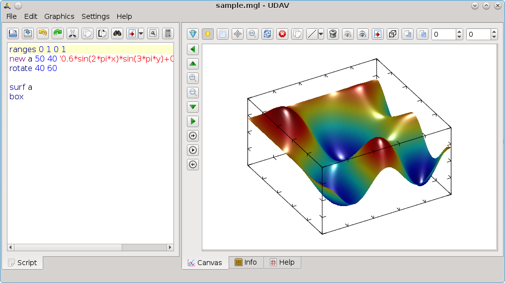
Main window is shown on the figure above. You can see the script (at left) with current line highlighted by light-yellow, and result of its execution at right. Each panel have its own set of toolbuttons.
Editor toolbuttons allow: open and save script from/to file; undo and redo changes; cut, copy and paste selection; find/replace text; show dialogs for command arguments and for plot setup; show calculator at bottom.
Graphics toolbuttons allow: enable/disable additional transparency and lighting; show grid of absolute coordinates; enable mouse rotation; restore image view; refresh graphics (execute the script); stop calculation; copy graphics into clipboard; add primitives (line, curve, box, rhombus, ellipse, mark, text) to the image; change view angles manually. Vertical toolbuttons allow: shift and zoom in/out of image as whole; show next and previous frame of animation, or start animation (if one present).
Graphics panel support plot editing by mouse.

Short command description and list of its arguments are shown at the status-bar, when you move cursor to the new line of code. You can press F1 to see more detailed help on special panel.

Also you can look the current list of variables, its dimensions and its size in the memory (right side of above figure). Toolbuttons allow: create new variable, edit variable, delete variable, preview variable plot and its properties, refresh list of variables. Pressing on any column will sort table according its contents. Double click on a variable will open panel with data cells of the variable, where you can view/edit each cell independently or apply a set of transformations.

Finally, pressing F2 or F4 you can show/hide windows with messages/warnings and with calculator. Double click on a warning in message window will jump to corresponding line in editor. Calculator allow you type expression by keyboard as well as by toolbuttons. It know about all current variables, so you can use them in formulas.
Next: UDAV hints, Previous: UDAV overview, Up: UDAV [Contents][Index]
There are a set of dialogs, which allow change/add a command, setup global plot properties, or setup UDAV itself.
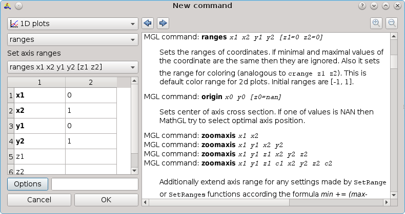
One of most interesting dialog (hotkey Meta-C or Win-C) is dialog which help to enter new command or change arguments of existed one. It allows consequently select the category of command, command name in category and appropriate set of command arguments. At this right side show detailed command description. Required argument(s) are denoted by bold text. Strings are placed in apostrophes, like 'txt'. Buttons below table allow to call dialogs for changing style of command (if argument 'fmt' is present in the list of command arguments); to set variable or expression for argument(s); to add options for command. Note, you can click on a cell to enter value, or double-click to call corresponding dialog.


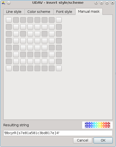
Dialog for changing style can be called independently, but usually is called from New command dialog or by double click on primitive. It contain 3 tabs: one for pen style, one for color scheme, one for text style. You should select appropriate one. Resulting string of style and sample picture are shown at bottom of dialog. Usually it can be called from New command dialog.

Dialog for entering variable allow to select variable or expression which can be used as argument of a command. Here you can select the variable name; range of indexes in each directions; operation which will be applied (like, summation, finding minimal/maximal values and so on). Usually it can be called from New command dialog.

Dialog for command options allow to change Command options. Usually it can be called from New command dialog.

Another interesting dialog, which help to select and properly setup a subplot, inplot, columnplot, stickplot and similar commands.


There is dialog for setting general plot properties, including tab for setting lighting properties. It can be called by called by hotkey ??? and put setup commands at the beginning of MGL script.
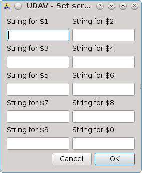
Also you can set or change script parameters (‘$0’ ... ‘$9’, see MGL definition).

Finally, there is dialog for UDAV settings. It allow to change most of things in UDAV appearance and working, including colors of keywords and numbers, default font and image size, and so on (see figure above).
There are also a set of dialogs for data handling, but they are too simple and clear. So, I will not put them here.
Previous: UDAV dialogs, Up: UDAV [Contents][Index]
mglconv, mglview.
Next: All samples, Previous: UDAV, Up: Top [Contents][Index]
There are few end-user classes: mglGraph (see MathGL core), mglWindow and mglGLUT (see Widget classes), mglData (see Data processing), mglParse (see MGL scripts). Exactly these classes I recommend to use in most of user programs. All methods in all of these classes are inline and have exact C/Fortran analogue functions. This give compiler independent binary libraries for MathGL.
However, sometimes you may need to extend MathGL by writing yours own plotting functions or handling yours own data structures. In these cases you may need to use low-level API. This chapter describes it.
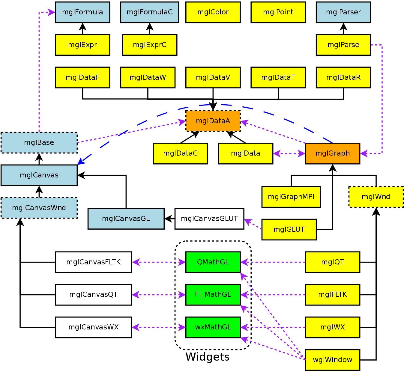
The internal structure of MathGL is rather complicated. There are C++ classes mglBase, mglCanvas, ... for drawing primitives and positioning the plot (blue ones in the figure). There is a layer of C functions, which include interface for most important methods of these classes. Also most of plotting functions are implemented as C functions. After it, there are “inline” front-end classes which are created for user convenience (yellow ones in the figure). Also there are widgets for FLTK and Qt libraries (green ones in the figure).
Below I show how this internal classes can be used.
| • mglBase class | ||
| • mglDataA class | ||
| • mglColor class | ||
| • mglPoint class |
Next: mglDataA class, Up: Other classes [Contents][Index]
Basically most of new kinds of plot can be created using just MathGL primitives (see Primitives). However the usage of mglBase methods can give you higher speed of drawing and better control of plot settings.
All plotting functions should use a pointer to mglBase class (or HMGL type in C functions) due to compatibility issues. Exactly such type of pointers are used in front-end classes (mglGraph, mglWindow) and in widgets (QMathGL, Fl_MathGL).
MathGL tries to remember all vertexes and all primitives and plot creation stage, and to use them for making final picture by demand. Basically for making plot, you need to add vertexes by AddPnt() function, which return index for new vertex, and call one of primitive drawing function (like mark_plot(), arrow_plot(), line_plot(), trig_plot(), quad_plot(), text_plot()), using vertex indexes as argument(s). AddPnt() function use 2 mreal numbers for color specification. First one is positioning in textures – integer part is texture index, fractional part is relative coordinate in the texture. Second number is like a transparency of plot (or second coordinate in the 2D texture).
I don’t want to put here detailed description of mglBase class. It was rather well documented in mgl2/base.h file. I just show and example of its usage on the base of circle drawing.
First, we should prototype new function circle() as C function.
#ifdef __cplusplus
extern "C" {
#endif
void circle(HMGL gr, mreal x, mreal y, mreal z, mreal r, const char *stl, const char *opt);
#ifdef __cplusplus
}
#endif
This is done for generating compiler independent binary. Because only C-functions have standard naming mechanism, the same for any compilers.
Now, we create a C++ file and put the code of function. I’ll write it line by line and try to comment all important points.
void circle(HMGL gr, mreal x, mreal y, mreal z, mreal r, const char *stl, const char *opt)
{
First, we need to check all input arguments and send warnings if something is wrong. In our case it is negative value of r argument. We just send warning, since it is not critical situation – other plot still can be drawn.
if(r<=0) { gr->SetWarn(mglWarnNeg,"Circle"); return; }
Next step is creating a group. Group keep some general setting for plot (like options) and useful for export in 3d files.
static int cgid=1; gr->StartGroup("Circle",cgid++);
Now let apply options. Options are rather useful things, generally, which allow one easily redefine axis range(s), transparency and other settings (see Command options).
gr->SaveState(opt);
I use global setting for determining the number of points in circle approximation. Note, that user can change MeshNum by options easily.
const int n = gr->MeshNum>1?gr->MeshNum : 41;
Let try to determine plot specific flags. MathGL functions expect that most of flags will be sent in string. In our case it is symbol ‘@’ which set to draw filled circle instead of border only (last will be default). Note, you have to handle NULL as string pointer.
bool fill = mglchr(stl,'@');
Now, time for coloring. I use palette mechanism because circle have few colors: one for filling and another for border. SetPenPal() function parse input string and write resulting texture index in pal. Function return the character for marker, which can be specified in string str. Marker will be plotted at the center of circle. I’ll show on next sample how you can use color schemes (smooth colors) too.
  long pal=0;
  char mk=gr->SetPenPal(stl,&pal);
Next step, is determining colors for filling and for border. First one for filling.
mreal c=gr->NextColor(pal), d;
Second one for border. I use black color (call gr->AddTexture('k')) if second color is not specified.
mreal k=(gr->GetNumPal(pal)>1)?gr->NextColor(pal):gr->AddTexture('k');
If user want draw only border (fill=false) then I use first color for border.
if(!fill) k=c;
Now we should reserve space for vertexes. This functions need n for border, n+1 for filling and 1 for marker. So, maximal number of vertexes is 2*n+2. Note, that such reservation is not required for normal work but can sufficiently speed up the plotting.
gr->Reserve(2*n+2);
We’ve done with setup and ready to start drawing. First, we need to add vertex(es). Let define NAN as normals, since I don’t want handle lighting for this plot,
mglPoint q(NAN,NAN);
and start adding vertexes. First one for central point of filling. I use -1 if I don’t need this point. The arguments of AddPnt() function is: mglPoint(x,y,z) – coordinate of vertex, c – vertex color, q – normal at vertex, -1 – vertex transparency (-1 for default), 3 bitwise flag which show that coordinates will be scaled (0x1) and will not be cutted (0x2).
  long n0,n1,n2,m1,m2,i;
  n0 = fill ? gr->AddPnt(mglPoint(x,y,z),c,q,-1,3):-1;
Similar for marker, but we use different color k.
n2 = mk ? gr->AddPnt(mglPoint(x,y,z),k,q,-1,3):-1;
Draw marker.
if(mk) gr->mark_plot(n2,mk);
Time for drawing circle itself. I use -1 for m1, n1 as sign that primitives shouldn’t be drawn for first point i=0.
  for(i=0,m1=n1=-1;i<n;i++)
  {
Each function should check Stop variable and return if it is non-zero. It is done for interrupting drawing for system which don’t support multi-threading.
if(gr->Stop) return;
Let find coordinates of vertex.
    mreal t = i*2*M_PI/(n-1.);
    mglPoint p(x+r*cos(t), y+r*sin(t), z);
Save previous vertex and add next one
n2 = n1; n1 = gr->AddPnt(p,c,q,-1,3);
and copy it for border but with different color. Such copying is much faster than adding new vertex using AddPnt().
m2 = m1; m1 = gr->CopyNtoC(n1,k);
Now draw triangle for filling internal part
if(fill) gr->trig_plot(n0,n1,n2);
and draw line for border.
    gr->line_plot(m1,m2);
  }
Drawing is done. Let close group and return.
  gr->EndGroup();
}
Another sample I want to show is exactly the same function but with smooth coloring using color scheme. So, I’ll add comments only in the place of difference.
void circle_cs(HMGL gr, mreal x, mreal y, mreal z, mreal r, const char *stl, const char *opt)
{
In this case let allow negative radius too. Formally it is not the problem for plotting (formulas the same) and this allow us to handle all color range.
//if(r<=0)  { gr->SetWarn(mglWarnNeg,"Circle"); return; }

  static int cgid=1;  gr->StartGroup("CircleCS",cgid++);
  gr->SaveState(opt);
  const int n = gr->MeshNum>1?gr->MeshNum : 41;
  bool fill = mglchr(stl,'@');
Here is main difference. We need to create texture for color scheme specified by user
long ss = gr->AddTexture(stl);
But we need also get marker and color for it (if filling is enabled). Let suppose that marker and color is specified after ‘:’. This is standard delimiter which stop color scheme entering. So, just lets find it and use for setting pen.
  const char *pen=0;
  if(stl) pen = strchr(stl,':');
  if(pen) pen++;
The substring is placed in pen and it will be used as line style.
  long pal=0;
  char mk=gr->SetPenPal(pen,&pal);
Next step, is determining colors for filling and for border. First one for filling.
mreal c=gr->GetC(ss,r);
Second one for border.
mreal k=gr->NextColor(pal);
The rest part is the same as in previous function.
  if(!fill) k=c;

  gr->Reserve(2*n+2);
  mglPoint q(NAN,NAN);
  long n0,n1,n2,m1,m2,i;
  n0 = fill ? gr->AddPnt(mglPoint(x,y,z),c,q,-1,3):-1;
  n2 = mk ? gr->AddPnt(mglPoint(x,y,z),k,q,-1,3):-1;
  if(mk)  gr->mark_plot(n2,mk);
  for(i=0,m1=n1=-1;i<n;i++)
  {
    if(gr->Stop)  return;
    mreal t = i*2*M_PI/(n-1.);
    mglPoint p(x+r*cos(t), y+r*sin(t), z);
    n2 = n1;  n1 = gr->AddPnt(p,c,q,-1,3);
    m2 = m1;  m1 = gr->CopyNtoC(n1,k);
    if(fill)  gr->trig_plot(n0,n1,n2);
    gr->line_plot(m1,m2);
  }
  gr->EndGroup();
}
The last thing which we can do is derive our own class with new plotting functions. Good idea is to derive it from mglGraph (if you don’t need extended window), or from mglWindow (if you need to extend window). So, in our case it will be
class MyGraph : public mglGraph
{
public:
  inline void Circle(mglPoint p, mreal r, const char *stl="", const char *opt="")
  { circle(p.x,p.y,p.z, r, stl, opt); }
  inline void CircleCS(mglPoint p, mreal r, const char *stl="", const char *opt="")
  { circle_cs(p.x,p.y,p.z, r, stl, opt); }
};
Note, that I use inline modifier for using the same binary code with different compilers.
So, the complete sample will be
#include <mgl2/mgl.h>
//---------------------------------------------------------
#ifdef __cplusplus
extern "C" {
#endif
void circle(HMGL gr, mreal x, mreal y, mreal z, mreal r, const char *stl, const char *opt);
void circle_cs(HMGL gr, mreal x, mreal y, mreal z, mreal r, const char *stl, const char *opt);
#ifdef __cplusplus
}
#endif
//---------------------------------------------------------
class MyGraph : public mglGraph
{
public:
  inline void CircleCF(mglPoint p, mreal r, const char *stl="", const char *opt="")
  { circle(p.x,p.y,p.z, r, stl, opt); }
  inline void CircleCS(mglPoint p, mreal r, const char *stl="", const char *opt="")
  { circle_cs(p.x,p.y,p.z, r, stl, opt); }
};
//---------------------------------------------------------
void circle(HMGL gr, mreal x, mreal y, mreal z, mreal r, const char *stl, const char *opt)
{
  if(r<=0)  { gr->SetWarn(mglWarnNeg,"Circle"); return; }
  static int cgid=1;  gr->StartGroup("Circle",cgid++);
  gr->SaveState(opt);
  const int n = gr->MeshNum>1?gr->MeshNum : 41;
  bool fill = mglchr(stl,'@');
  long pal=0;
  char mk=gr->SetPenPal(stl,&pal);
  mreal c=gr->NextColor(pal), d;
  mreal k=(gr->GetNumPal(pal)>1)?gr->NextColor(pal):gr->AddTexture('k');
  if(!fill) k=c;
  gr->Reserve(2*n+2);
  mglPoint q(NAN,NAN);
  long n0,n1,n2,m1,m2,i;
  n0 = fill ? gr->AddPnt(mglPoint(x,y,z),c,q,-1,3):-1;
  n2 = mk ? gr->AddPnt(mglPoint(x,y,z),k,q,-1,3):-1;
  if(mk)  gr->mark_plot(n2,mk);
  for(i=0,m1=n1=-1;i<n;i++)
  {
    if(gr->Stop)  return;
    mreal t = i*2*M_PI/(n-1.);
    mglPoint p(x+r*cos(t), y+r*sin(t), z);
    n2 = n1;  n1 = gr->AddPnt(p,c,q,-1,3);
    m2 = m1;  m1 = gr->CopyNtoC(n1,k);
    if(fill)  gr->trig_plot(n0,n1,n2);
    gr->line_plot(m1,m2);
  }
  gr->EndGroup();
}
//---------------------------------------------------------
void circle_cs(HMGL gr, mreal x, mreal y, mreal z, mreal r, const char *stl, const char *opt)
{
  static int cgid=1;  gr->StartGroup("CircleCS",cgid++);
  gr->SaveState(opt);
  const int n = gr->MeshNum>1?gr->MeshNum : 41;
  bool fill = mglchr(stl,'@');
  long ss = gr->AddTexture(stl);
  const char *pen=0;
  if(stl) pen = strchr(stl,':');
  if(pen) pen++;
  long pal=0;
  char mk=gr->SetPenPal(pen,&pal);
  mreal c=gr->GetC(ss,r);
  mreal k=gr->NextColor(pal);
  if(!fill) k=c;

  gr->Reserve(2*n+2);
  mglPoint q(NAN,NAN);
  long n0,n1,n2,m1,m2,i;
  n0 = fill ? gr->AddPnt(mglPoint(x,y,z),c,q,-1,3):-1;
  n2 = mk ? gr->AddPnt(mglPoint(x,y,z),k,q,-1,3):-1;
  if(mk)  gr->mark_plot(n2,mk);
  for(i=0,m1=n1=-1;i<n;i++)
  {
    if(gr->Stop)  return;
    mreal t = i*2*M_PI/(n-1.);
    mglPoint p(x+r*cos(t), y+r*sin(t), z);
    n2 = n1;  n1 = gr->AddPnt(p,c,q,-1,3);
    m2 = m1;  m1 = gr->CopyNtoC(n1,k);
    if(fill)  gr->trig_plot(n0,n1,n2);
    gr->line_plot(m1,m2);
  }
  gr->EndGroup();
}
//---------------------------------------------------------
int main()
{
  MyGraph gr;
  gr.Box();
  // first let draw circles with fixed colors
  for(int i=0;i<10;i++)
    gr.CircleCF(mglPoint(2*mgl_rnd()-1, 2*mgl_rnd()-1), mgl_rnd());
  // now let draw circles with color scheme
  for(int i=0;i<10;i++)
    gr.CircleCS(mglPoint(2*mgl_rnd()-1, 2*mgl_rnd()-1), 2*mgl_rnd()-1);
}
Next: mglColor class, Previous: mglBase class, Up: Other classes [Contents][Index]
mglData class have abstract predecessor class mglDataA. Exactly the pointers to mglDataA instances are used in all plotting functions and some of data processing functions. This was done for taking possibility to define yours own class, which will handle yours own data (for example, complex numbers, or differently organized data). And this new class will be almost the same as mglData for plotting purposes.
However, the most of data processing functions will be slower as if you used mglData instance. This is more or less understandable – I don’t know how data in yours particular class will be organized, and couldn’t optimize the these functions generally.
There are few virtual functions which must be provided in derived classes. This functions give:
GetNx, GetNy, GetNz),
v, dvx, dvy, dvz),
Maximal, Minimal) – you can use provided functions (like mgl_data_max and mgl_data_min), but yours own realization can be more efficient,
vthr) – you need this only if you want using MathGL’s data processing functions.
Let me, for example define class mglComplex which will handle complex number and draw its amplitude or phase, depending on flag use_abs:
#include <complex>
#include <mgl2/mgl.h>
#define dual std::complex<double>
class mglComplex : public mglDataA
{
public:
  long nx;      ///< number of points in 1st dimensions ('x' dimension)
  long ny;      ///< number of points in 2nd dimensions ('y' dimension)
  long nz;      ///< number of points in 3d dimensions ('z' dimension)
  dual *a;      ///< data array
  bool use_abs; ///< flag to use abs() or arg()

  inline mglComplex(long xx=1,long yy=1,long zz=1)
  { a=0;  use_abs=true; Create(xx,yy,zz); }
  virtual ~mglComplex()  { if(a)  delete []a; }

  /// Get sizes
  inline long GetNx() const { return nx;  }
  inline long GetNy() const { return ny;  }
  inline long GetNz() const { return nz;  }
  /// Create or recreate the array with specified size and fill it by zero
  inline void Create(long mx,long my=1,long mz=1)
  { nx=mx;  ny=my;  nz=mz;  if(a) delete []a;
  a = new dual[nx*ny*nz]; }
  /// Get maximal value of the data
  inline mreal Maximal() const  { return mgl_data_max(this);  }
  /// Get minimal value of the data
  inline mreal Minimal() const  { return mgl_data_min(this);  }

protected:
  inline mreal v(long i,long j=0,long k=0) const
  { return use_abs ? abs(a[i+nx*(j+ny*k)]) : arg(a[i+nx*(j+ny*k)]);  }
  inline mreal vthr(long i) const
  { return use_abs ? abs(a[i]) : arg(a[i]);  }
  inline mreal dvx(long i,long j=0,long k=0) const
  { long i0=i+nx*(j+ny*k);
    std::complex<double> res=i>0? (i<nx-1? (a[i0+1]-a[i0-1])/2.:a[i0]-a[i0-1]) : a[i0+1]-a[i0];
    return use_abs? abs(res) : arg(res);  }
  inline mreal dvy(long i,long j=0,long k=0) const
  { long i0=i+nx*(j+ny*k);
    std::complex<double> res=j>0? (j<ny-1? (a[i0+nx]-a[i0-nx])/2.:a[i0]-a[i0-nx]) : a[i0+nx]-a[i0];
    return use_abs? abs(res) : arg(res);  }
  inline mreal dvz(long i,long j=0,long k=0) const
  { long i0=i+nx*(j+ny*k), n=nx*ny;
    std::complex<double> res=k>0? (k<nz-1? (a[i0+n]-a[i0-n])/2.:a[i0]-a[i0-n]) : a[i0+n]-a[i0];
    return use_abs? abs(res) : arg(res);  }
};
int main()
{
  mglComplex dat(20);
  for(long i=0;i<20;i++)
    dat.a[i] = 3*exp(-0.05*(i-10)*(i-10))*dual(cos(M_PI*i*0.3), sin(M_PI*i*0.3));
  mglGraph gr;
  gr.SetRange('y', -M_PI, M_PI);  gr.Box();

  gr.Plot(dat,"r","legend 'abs'");
  dat.use_abs=false;
  gr.Plot(dat,"b","legend 'arg'");
  gr.Legend();
  gr.WritePNG("complex.png");
  return 0;
}
Next: mglPoint class, Previous: mglDataA class, Up: Other classes [Contents][Index]
Structure for working with colors. This structure is defined in #include <mgl2/type.h>.
There are two ways to set the color in MathGL. First one is using of mreal values of red, green and blue channels for precise color definition. The second way is the using of character id. There are a set of characters specifying frequently used colors. Normally capital letter gives more dark color than lowercase one. See Line styles.
mreal r, g, b, aReg, green and blue component of color.
mreal R, mreal G, mreal B, mreal A=1)Constructor sets the color by mreal values of Red, Green, Blue and Alpha channels. These values should be in interval [0,1].
char c='k', mreal bright=1)Constructor sets the color from character id. The black color is used by default. Parameter br set additional “lightness” of color.
void Set (mreal R, mreal G, mreal B, mreal A=1)Sets color from values of Red, Green, Blue and Alpha channels. These values should be in interval [0,1].
void Set (mglColor c, mreal bright=1)Sets color as “lighted” version of color c.
void Set (char p, mreal bright=1)Sets color from symbolic id.
bool Valid ()Checks correctness of the color.
mreal Norm ()Gets maximal of spectral component.
bool operator== (const mglColor &c)bool operator!= (const mglColor &c)Compare with another color
bool operator*= (mreal v)Multiplies color components by number v.
bool operator+= (const mglColor &c)Adds color c component by component.
bool operator-= (const mglColor &c)Subtracts color c component by component.
const mglColor &a, const mglColor &b)Adds colors by its RGB values.
mglColor operator- (const mglColor &a, const mglColor &b)Subtracts colors by its RGB values.
mglColor operator* (const mglColor &a, mreal b)mglColor operator* (mreal a, const mglColor &b)Multiplies color by number.
mglColor operator/ (const mglColor &a, mreal b)Divide color by number.
mglColor operator! (const mglColor &a)Return inverted color.
Previous: mglColor class, Up: Other classes [Contents][Index]
Structure describes point in space. This structure is defined in #include <mgl2/type.h>
mreal x, y, z, cPoint coordinates {x,y,z} and one extra value c used for amplitude, transparency and so on. By default all values are zero.
mreal X=0, mreal Y=0, mreal Z=0, mreal C=0)Constructor sets the color by mreal values of Red, Green, Blue and Alpha channels. These values should be in interval [0,1].
bool IsNAN ()Returns true if point contain NAN values.
mreal norm ()Returns the norm \sqrt{x^2+y^2+z^2} of vector.
void Normalize ()Normalizes vector to be unit vector.
mreal val (int i)Returns point component: x for i=0, y for i=1, z for i=2, c for i=3.
mglPoint operator+ (const mglPoint &a, const mglPoint &b)Point of summation (summation of vectors).
mglPoint operator- (const mglPoint &a, const mglPoint &b)Point of difference (difference of vectors).
mglPoint operator* (mreal a, const mglPoint &b)mglPoint operator* (const mglPoint &a, mreal b)Multiplies (scale) points by number.
mglPoint operator/ (const mglPoint &a, mreal b)Multiplies (scale) points by number 1/b.
mreal operator* (const mglPoint &a, const mglPoint &b)Scalar product of vectors.
mglPoint operator/ (const mglPoint &a, const mglPoint &b)Return vector of element-by-element product.
mglPoint operator^ (const mglPoint &a, const mglPoint &b)Cross-product of vectors.
mglPoint operator& (const mglPoint &a, const mglPoint &b)The part of a which is perpendicular to vector b.
mglPoint operator| (const mglPoint &a, const mglPoint &b)The part of a which is parallel to vector b.
mglPoint operator! (const mglPoint &a)Return vector perpendicular to vector a.
mreal mgl_norm (const mglPoint &a)Return the norm sqrt(|a|^2) of vector a.
bool operator== (const mglPoint &a, const mglPoint &b)Return true if points are the same.
bool operator!= (const mglPoint &a, const mglPoint &b)Return true if points are different.
Next: Symbols and hot-keys, Previous: Other classes, Up: Top [Contents][Index]
This chapter contain alphabetical list of MGL and C++ samples for most of MathGL graphics and features.
Next: 3wave sample, Up: All samples [Contents][Index]
This section contain functions for input data for most of further samples.
MGL code:
func 'prepare1d'
new y 50 3
modify y '0.7*sin(2*pi*x)+0.5*cos(3*pi*x)+0.2*sin(pi*x)'
modify y 'sin(2*pi*x)' 1
modify y 'cos(2*pi*x)' 2
new x1 50 'x'
new x2 50 '0.05-0.03*cos(pi*x)'
new y1 50 '0.5-0.3*cos(pi*x)'
new y2 50 '-0.3*sin(pi*x)'
return

func 'prepare2d'
new a 50 40 '0.6*sin(pi*(x+1))*sin(1.5*pi*(y+1))+0.4*cos(0.75*pi*(x+1)*(y+1))'
new b 50 40 '0.6*cos(pi*(x+1))*cos(1.5*pi*(y+1))+0.4*cos(0.75*pi*(x+1)*(y+1))'
return

func 'prepare3d'
new c 61 50 40 '-2*(x^2+y^2+z^4-z^2)+0.2'
new d 61 50 40 '1-2*tanh((x+y)*(x+y))'
return

func 'prepare2v'
new a 20 30 '0.6*sin(pi*(x+1))*sin(1.5*pi*(y+1))+0.4*cos(0.75*pi*(x+1)*(y+1))'
new b 20 30 '0.6*cos(pi*(x+1))*cos(1.5*pi*(y+1))+0.4*cos(0.75*pi*(x+1)*(y+1))'
return

func 'prepare3v'
define $1 pow(x*x+y*y+(z-0.3)*(z-0.3)+0.03,1.5)
define $2 pow(x*x+y*y+(z+0.3)*(z+0.3)+0.03,1.5)
new ex 10 10 10 '0.2*x/$1-0.2*x/$2'
new ey 10 10 10 '0.2*y/$1-0.2*y/$2'
new ez 10 10 10 '0.2*(z-0.3)/$1-0.2*(z+0.3)/$2'
return
C++ code:
void mgls_prepare1d(mglData *y, mglData *y1, mglData *y2, mglData *x1, mglData *x2)
{
	long n=50;
	if(y)	y->Create(n,3);
	if(x1)	x1->Create(n);
	if(x2)	x2->Create(n);
	if(y1)	y1->Create(n);
	if(y2)	y2->Create(n);
	for(long i=0;i<n;i++)
	{
		double xx = i/(n-1.);
		if(y)
		{
			y->a[i] = 0.7*sin(2*M_PI*xx) + 0.5*cos(3*M_PI*xx) + 0.2*sin(M_PI*xx);
			y->a[i+n] = sin(2*M_PI*xx);
			y->a[i+2*n] = cos(2*M_PI*xx);
		}
		if(y1)	y1->a[i] = 0.5+0.3*cos(2*M_PI*xx);
		if(y2)	y2->a[i] = 0.3*sin(2*M_PI*xx);
		if(x1)	x1->a[i] = xx*2-1;
		if(x2)	x2->a[i] = 0.05+0.03*cos(2*M_PI*xx);
	}
}
//-----------------------------------------------------------------------------
void mgls_prepare2d(mglData *a, mglData *b, mglData *v)
{
	long n=50,m=40;
	if(a)	a->Create(n,m);
	if(b)	b->Create(n,m);
	if(v)	{	v->Create(9);	v->Fill(-1,1);	}
	for(long j=0;j<m;j++)	for(long i=0;i<n;i++)
	{
		double x = i/(n-1.), y = j/(m-1.);
		long i0 = i+n*j;
		if(a)	a->a[i0] = 0.6*sin(2*M_PI*x)*sin(3*M_PI*y)+0.4*cos(3*M_PI*x*y);
		if(b)	b->a[i0] = 0.6*cos(2*M_PI*x)*cos(3*M_PI*y)+0.4*cos(3*M_PI*x*y);
	}
}
//-----------------------------------------------------------------------------
void mgls_prepare3d(mglData *a, mglData *b)
{
	long n=61,m=50,l=40;
	if(a)	a->Create(n,m,l);
	if(b)	b->Create(n,m,l);
	for(long k=0;k<l;k++)	for(long j=0;j<m;j++)	for(long i=0;i<n;i++)
	{
		double x=2*i/(n-1.)-1, y=2*j/(m-1.)-1, z=2*k/(l-1.)-1;
		long i0 = i+n*(j+m*k);
		if(a)	a->a[i0] = -2*(x*x + y*y + z*z*z*z - z*z - 0.1);
		if(b)	b->a[i0] = 1-2*tanh((x+y)*(x+y));
	}
}
//-----------------------------------------------------------------------------
void mgls_prepare2v(mglData *a, mglData *b)
{
	long n=20,m=30;
	if(a)	a->Create(n,m);
	if(b)	b->Create(n,m);
	for(long j=0;j<m;j++)	for(long i=0;i<n;i++)
	{
		double x=i/(n-1.), y=j/(m-1.);
		long i0 = i+n*j;
		if(a)	a->a[i0] = 0.6*sin(2*M_PI*x)*sin(3*M_PI*y)+0.4*cos(3*M_PI*x*y);
		if(b)	b->a[i0] = 0.6*cos(2*M_PI*x)*cos(3*M_PI*y)+0.4*cos(3*M_PI*x*y);
	}
}
//-----------------------------------------------------------------------------
void mgls_prepare3v(mglData *ex, mglData *ey, mglData *ez)
{
	long n=10;
	double z0=0.3;
	if(!ex || !ey || !ez)	return;
	ex->Create(n,n,n);	ey->Create(n,n,n);	ez->Create(n,n,n);
	for(long k=0;k<n;k++)	for(long j=0;j<n;j++)	for(long i=0;i<n;i++)
	{
		double x=2*i/(n-1.)-1, y=2*j/(n-1.)-1, z=2*k/(n-1.)-1;
		long i0 = i+n*(j+k*n);
		double r1 = pow(x*x+y*y+(z-z0)*(z-z0)+0.03,1.5);
		double r2 = pow(x*x+y*y+(z+z0)*(z+z0)+0.03,1.5);
		ex->a[i0]=0.2*x/r1 - 0.2*x/r2;
		ey->a[i0]=0.2*y/r1 - 0.2*y/r2;
		ez->a[i0]=0.2*(z-z0)/r1 - 0.2*(z+z0)/r2;
	}
}
//-----------------------------------------------------------------------------
Next: alpha sample, Previous: initialization sample, Up: All samples [Contents][Index]
Example of complex ode on basis of 3-wave decay.
MGL code:
define t 50
ode !r '-b*f;a*conj(f);a*conj(b)-0.1*f' 'abf' [1,1e-3,0] 0.1 t
ranges 0 t 0 r.max
plot r(0) 'b';legend 'a'
plot r(1) 'g';legend 'b'
plot r(2) 'r';legend 'f'
axis:box:legend
C++ code:
void smgl_3wave(mglGraph *gr)
{
	gr->SubPlot(1,1,0,"<_");
	if(big!=3)	gr->Title("Complex ODE sample");
	double t=50;
	mglData ini;	ini.SetList(3, 1., 1e-3, 0.);
	mglDataC r(mglODEc("-b*f;a*conj(f);a*conj(b)-0.1*f","abf",ini,0.1,t));
	gr->SetRanges(0, t, 0, r.Maximal());
	gr->Plot(r.SubData(0),"b","legend 'a'");
	gr->Plot(r.SubData(1),"g","legend 'b'");
	gr->Plot(r.SubData(2),"r","legend 'f'");
	gr->Axis();	gr->Box();	gr->Legend();
}
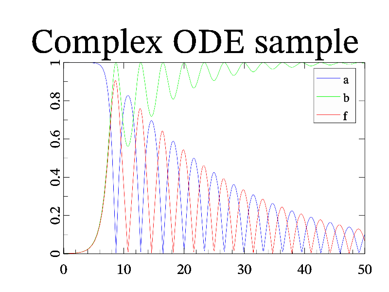
Next: apde sample, Previous: 3wave sample, Up: All samples [Contents][Index]
Example of light and alpha (transparency).
MGL code:
call 'prepare2d'
subplot 2 2 0:title 'default':rotate 50 60:box
surf a
subplot 2 2 1:title 'light on':rotate 50 60:box
light on:surf a
subplot 2 2 3:title 'light on; alpha on':rotate 50 60:box
alpha on:surf a
subplot 2 2 2:title 'alpha on':rotate 50 60:box
light off:surf a
C++ code:
void smgl_alpha(mglGraph *gr)	// alpha and lighting
{
	mglData a;	mgls_prepare2d(&a);
	gr->SubPlot(2,2,0);	gr->Title("default");	gr->Rotate(50,60);
	gr->Box();	gr->Surf(a);
	gr->SubPlot(2,2,1);	gr->Title("light on");	gr->Rotate(50,60);
	gr->Box();	gr->Light(true);	gr->Surf(a);
	gr->SubPlot(2,2,3);	gr->Title("alpha on; light on");	gr->Rotate(50,60);
	gr->Box();	gr->Alpha(true);	gr->Surf(a);
	gr->SubPlot(2,2,2);	gr->Title("alpha on");	gr->Rotate(50,60);
	gr->Box();	gr->Light(false);	gr->Surf(a);
}
Next: area sample, Previous: alpha sample, Up: All samples [Contents][Index]
Comparison of advanced PDE solver (apde) and ordinary one (pde).
MGL code:
ranges -1 1 0 2 0 2
new ar 256 'exp(-2*(x+0.0)^2)'
new ai 256

apde res1 'exp(-x^2-p^2)' ar ai 0.01:transpose res1
pde res2 'exp(-x^2-p^2)' ar ai 0.01

subplot 1 2 0 '_':title 'Advanced PDE solver'
ranges 0 2 -1 1:crange res1
dens res1:box
axis:xlabel '\i z':ylabel '\i x'
text -0.5 0.2 'i\partial_z\i u = exp(-\i x^2+\partial_x^2)[\i u]' 'y'

subplot 1 2 1 '_':title 'Simplified PDE solver'
dens res2:box
axis:xlabel '\i z':ylabel '\i x'
text -0.5 0.2 'i\partial_z\i u \approx\ exp(-\i x^2)\i u+exp(\partial_x^2)[\i u]' 'y'
C++ code:
void smgl_apde(mglGraph *gr)
{
	gr->SetRanges(-1,1,0,2,0,2);
	mglData ar(256), ai(256);	gr->Fill(ar,"exp(-2*(x+0.0)^2)");

	mglData res1(gr->APDE("exp(-x^2-p^2)",ar,ai,0.01));	res1.Transpose();
	mglData res2(gr->PDE("exp(-x^2-p^2)",ar,ai,0.01));

	gr->SubPlot(1,2,0,"_");	gr->Title("Advanced PDE solver");
	gr->SetRanges(0,2,-1,1);	gr->SetRange('c',res1);
	gr->Dens(res1);	gr->Axis();	gr->Box();
	gr->Label('x',"\\i z");	gr->Label('y',"\\i x");
	gr->Puts(mglPoint(-0.5,0.2),"i\\partial_z\\i u = exp(-\\i x^2+\\partial_x^2)[\\i u]","y");

	gr->SubPlot(1,2,1,"_");	gr->Title("Simplified PDE solver");
	gr->Dens(res2);	gr->Axis();	gr->Box();
	gr->Label('x',"\\i z");	gr->Label('y',"\\i x");
	gr->Puts(mglPoint(-0.5,0.2),"i\\partial_z\\i u \\approx\\ exp(-\\i x^2)\\i u+exp(\\partial_x^2)[\\i u]","y");
}
Next: aspect sample, Previous: apde sample, Up: All samples [Contents][Index]
Function area fill the area between curve and axis plane. It support gradient filling if 2 colors per curve is specified.
MGL code:
call 'prepare1d'
origin 0 0 0
subplot 2 2 0 '':title 'Area plot (default)':box:area y
subplot 2 2 1 '':title '2 colors':box:area y 'cbgGyr'
subplot 2 2 2 '':title '"!" style':box:area y '!'
new yc 30 'sin(pi*x)':new xc 30 'cos(pi*x)':new z 30 'x'
subplot 2 2 3:title '3d variant':rotate 50 60:box
area xc yc z 'r'
area xc -yc z 'b#'
C++ code:
void smgl_area(mglGraph *gr)
{
	mglData y;	mgls_prepare1d(&y);	gr->SetOrigin(0,0,0);
	if(big!=3)	{	gr->SubPlot(2,2,0,"");	gr->Title("Area plot (default)");	}
	gr->Box();	gr->Area(y);
	if(big==3)	return;
	gr->SubPlot(2,2,1,"");	gr->Title("2 colors");	gr->Box();	gr->Area(y,"cbgGyr");
	gr->SubPlot(2,2,2,"");	gr->Title("'!' style");	gr->Box();	gr->Area(y,"!");
	gr->SubPlot(2,2,3);	gr->Title("3d variant");	gr->Rotate(50,60);	gr->Box();
	mglData yc(30), xc(30), z(30);	z.Modify("2*x-1");
	yc.Modify("sin(pi*(2*x-1))");	xc.Modify("cos(pi*2*x-pi)");
	gr->Area(xc,yc,z,"r");
	yc.Modify("-sin(pi*(2*x-1))");	gr->Area(xc,yc,z,"b#");
}
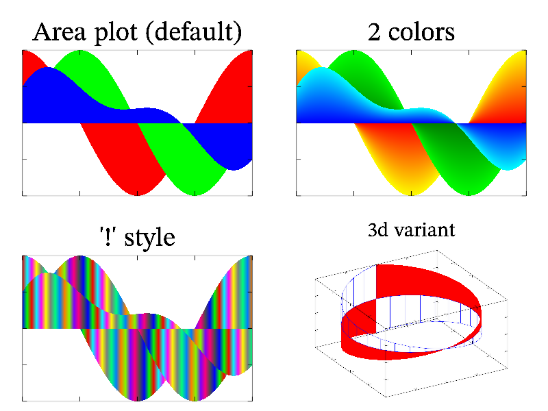
Next: axial sample, Previous: area sample, Up: All samples [Contents][Index]
Example of subplot, inplot, rotate, aspect, shear.
MGL code:
subplot 2 2 0:box:text -1 1.1 'Just box' ':L'
inplot 0.2 0.5 0.7 1 off:box:text 0 1.2 'InPlot example'
subplot 2 2 1:title 'Rotate only':rotate 50 60:box
subplot 2 2 2:title 'Rotate and Aspect':rotate 50 60:aspect 1 1 2:box
subplot 2 2 3:title 'Shear':box 'c':shear 0.2 0.1:box
C++ code:
void smgl_aspect(mglGraph *gr)	// transformation
{
	gr->SubPlot(2,2,0);	gr->Box();
	gr->Puts(mglPoint(-1,1.1),"Just box",":L");
	gr->InPlot(0.2,0.5,0.7,1,false);	gr->Box();
	gr->Puts(mglPoint(0,1.2),"InPlot example");
	gr->SubPlot(2,2,1);	gr->Title("Rotate only");
	gr->Rotate(50,60);	gr->Box();
	gr->SubPlot(2,2,2);	gr->Title("Rotate and Aspect");
	gr->Rotate(50,60);	gr->Aspect(1,1,2);	gr->Box();
	gr->SubPlot(2,2,3);	gr->Title("Shear");
	gr->Box("c");		gr->Shear(0.2,0.1);	gr->Box();
}
Next: axis sample, Previous: aspect sample, Up: All samples [Contents][Index]
Function axial draw surfaces of rotation for contour lines. You can draw wire surfaces (‘#’ style) or ones rotated in other directions (‘x’, ‘z’ styles).
MGL code:
call 'prepare2d'
subplot 2 2 0:title 'Axial plot (default)':light on:alpha on:rotate 50 60:box:axial a
subplot 2 2 1:title '"x" style;"." style':light on:rotate 50 60:box:axial a 'x.'
subplot 2 2 2:title '"z" style':light on:rotate 50 60:box:axial a 'z'
subplot 2 2 3:title '"\#" style':light on:rotate 50 60:box:axial a '#'
C++ code:
void smgl_axial(mglGraph *gr)
{
	mglData a;	mgls_prepare2d(&a);
	if(big!=3)	{	gr->SubPlot(2,2,0);	gr->Title("Axial plot (default)");	}
	gr->Light(true);	gr->Alpha(true);	gr->Rotate(50,60);	gr->Box();	gr->Axial(a);
	if(big==3)	return;
	gr->SubPlot(2,2,1);	gr->Title("'x' style; '.'style");	gr->Rotate(50,60);	gr->Box();	gr->Axial(a,"x.");
	gr->SubPlot(2,2,2);	gr->Title("'z' style");	gr->Rotate(50,60);	gr->Box();	gr->Axial(a,"z");
	gr->SubPlot(2,2,3);	gr->Title("'\\#' style");	gr->Rotate(50,60);	gr->Box();	gr->Axial(a,"#");
}
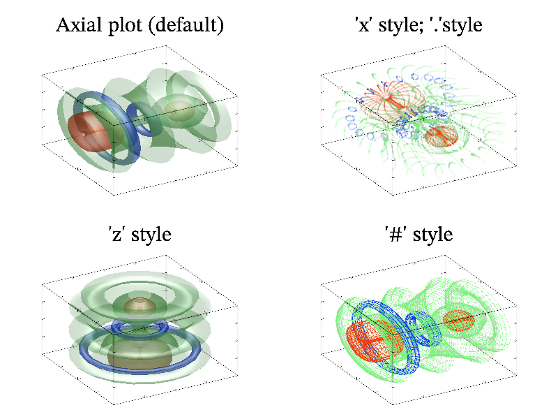
Next: background sample, Previous: axial sample, Up: All samples [Contents][Index]
Different forms of axis position.
MGL code:
subplot 2 2 0:title 'Axis origin, Grid':origin 0 0:axis:grid:fplot 'x^3'
subplot 2 2 1:title '2 axis':ranges -1 1 -1 1:origin -1 -1:axis:ylabel 'axis_1':fplot 'sin(pi*x)' 'r2'
ranges 0 1 0 1:origin 1 1:axis:ylabel 'axis_2':fplot 'cos(pi*x)'
subplot 2 2 3:title 'More axis':origin nan nan:xrange -1 1:axis:xlabel 'x' 0:ylabel 'y_1' 0:fplot 'x^2' 'k'
yrange -1 1:origin -1.3 -1:axis 'y' 'r':ylabel '#r{y_2}' 0.2:fplot 'x^3' 'r'

subplot 2 2 2:title '4 segments, inverted axis':origin 0 0:
inplot 0.5 1 0.5 1 on:ranges 0 10 0 2:axis
fplot 'sqrt(x/2)':xlabel 'W' 1:ylabel 'U' 1
inplot 0 0.5 0.5 1 on:ranges 1 0 0 2:axis 'x':fplot 'sqrt(x)+x^3':xlabel '\tau' 1
inplot 0.5 1 0 0.5 on:ranges 0 10 4 0:axis 'y':fplot 'x/4':ylabel 'L' -1
inplot 0 0.5 0 0.5 on:ranges 1 0 4 0:fplot '4*x^2'
C++ code:
void smgl_axis(mglGraph *gr)
{
	gr->SubPlot(2,2,0);	gr->Title("Axis origin, Grid");	gr->SetOrigin(0,0);
	gr->Axis();	gr->Grid();	gr->FPlot("x^3");

	gr->SubPlot(2,2,1);	gr->Title("2 axis");
	gr->SetRanges(-1,1,-1,1);	gr->SetOrigin(-1,-1,-1);	// first axis
	gr->Axis();	gr->Label('y',"axis 1",0);	gr->FPlot("sin(pi*x)","r2");
	gr->SetRanges(0,1,0,1);		gr->SetOrigin(1,1,1);		// second axis
	gr->Axis();	gr->Label('y',"axis 2",0);	gr->FPlot("cos(pi*x)");

	gr->SubPlot(2,2,3);	gr->Title("More axis");	gr->SetOrigin(NAN,NAN);	gr->SetRange('x',-1,1);
	gr->Axis();	gr->Label('x',"x",0);	gr->Label('y',"y_1",0);	gr->FPlot("x^2","k");
	gr->SetRanges(-1,1,-1,1);	gr->SetOrigin(-1.3,-1);	// second axis
	gr->Axis("y","r");	gr->Label('y',"#r{y_2}",0.2);	gr->FPlot("x^3","r");

	gr->SubPlot(2,2,2);	gr->Title("4 segments, inverted axis");		gr->SetOrigin(0,0);
	gr->InPlot(0.5,1,0.5,1);	gr->SetRanges(0,10,0,2);	gr->Axis();
	gr->FPlot("sqrt(x/2)");		gr->Label('x',"W",1);	gr->Label('y',"U",1);
	gr->InPlot(0,0.5,0.5,1);	gr->SetRanges(1,0,0,2);	gr->Axis("x");
	gr->FPlot("sqrt(x)+x^3");	gr->Label('x',"\\tau",-1);
	gr->InPlot(0.5,1,0,0.5);	gr->SetRanges(0,10,4,0);	gr->Axis("y");
	gr->FPlot("x/4");	gr->Label('y',"L",-1);
	gr->InPlot(0,0.5,0,0.5);	gr->SetRanges(1,0,4,0);	gr->FPlot("4*x^2");
}
Next: barh sample, Previous: axis sample, Up: All samples [Contents][Index]
Load background from an image file.
MGL code:
define $f udav_new.png
#background '$f' 's'
subplot 2 2 0 '':box
background '$f' 'a'
text 0.5 0.1 'Default' 'a'
subplot 2 2 1 '':box
background '$f' 'ca'
text 0.5 0.1 'Centering' 'a'
subplot 2 2 2 '':box
background '$f' 'ma'
text 0.5 0.1 'Mosaic' 'a'
subplot 2 2 3 '':box
background '$f' 'sa'
text 0.5 0.1 'Scaling' 'a'
C++ code:
void smgl_background(mglGraph *gr)
{
	const char *fname = "udav_new.png";
	gr->SubPlot(2,2,0,"");	gr->Box();	gr->LoadBackground(fname,"a");	gr->Puts(0.5,0.1,"Default","a");
	gr->SubPlot(2,2,1,"");	gr->Box();	gr->LoadBackground(fname,"ca");	gr->Puts(0.5,0.1,"Centering","a");
	gr->SubPlot(2,2,2,"");	gr->Box();	gr->LoadBackground(fname,"ma");	gr->Puts(0.5,0.1,"Mosaic","a");
	gr->SubPlot(2,2,3,"");	gr->Box();	gr->LoadBackground(fname,"sa");	gr->Puts(0.5,0.1,"Scaling","a");
	//gr->LoadBackground(fname,"s");
}
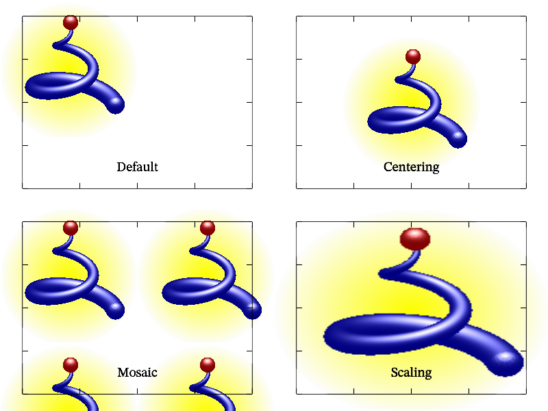
Next: bars sample, Previous: background sample, Up: All samples [Contents][Index]
Function barh is the similar to bars but draw horizontal bars.
MGL code:
new ys 10 3 '0.8*sin(pi*(x+y/4+1.25))+0.2*rnd':origin 0 0 0
subplot 2 2 0 '':title 'Barh plot (default)':box:barh ys
subplot 2 2 1 '':title '2 colors':box:barh ys 'cbgGyr'
ranges -3 3 -1 1:subplot 2 2 2 '':title '"a" style':box:barh ys 'a'
subplot 2 2 3 '': title '"f" style':box:barh ys 'f'
C++ code:
void smgl_barh(mglGraph *gr)
{
	mglData ys(10,3);	ys.Modify("0.8*sin(pi*(2*x+y/2))+0.2*rnd");
	gr->SetOrigin(0,0,0);
	if(big!=3)	{	gr->SubPlot(2,2,0,"");	gr->Title("Barh plot (default)");	}
	gr->Box();	gr->Barh(ys);
	if(big==3)	return;
	gr->SubPlot(2,2,1,"");	gr->Title("2 colors");	gr->Box();	gr->Barh(ys,"cbgGyr");
	gr->SetRanges(-3,3,-1,1);	// increase range since summation can exceed [-1,1]
	gr->SubPlot(2,2,2,"");	gr->Title("'a' style");	gr->Box();	gr->Barh(ys,"a");
	gr->SubPlot(2,2,3,"");	gr->Title("'f' style");	gr->Box();	gr->Barh(ys,"f");
}

Next: belt sample, Previous: barh sample, Up: All samples [Contents][Index]
Function bars draw vertical bars. It have a lot of options: bar-above-bar (‘a’ style), fall like (‘f’ style), 2 colors for positive and negative values, wired bars (‘#’ style), 3D variant.
MGL code:
new ys 10 3 '0.8*sin(pi*(x+y/4+1.25))+0.2*rnd':origin 0 0 0
subplot 3 2 0 '':title 'Bars plot (default)':box:bars ys
subplot 3 2 1 '':title '2 colors':box:bars ys 'cbgGyr'
subplot 3 2 4 '':title '"\#" style':box:bars ys '#'
new yc 30 'sin(pi*x)':new xc 30 'cos(pi*x)':new z 30 'x'
subplot 3 2 5:title '3d variant':rotate 50 60:box:bars xc yc z 'r'
ranges -1 1 -3 3:subplot 3 2 2 '':title '"a" style':box:bars ys 'a'
subplot 3 2 3 '':title '"f" style':box:bars ys 'f'
C++ code:
void smgl_bars(mglGraph *gr)
{
	mglData ys(10,3);	ys.Modify("0.8*sin(pi*(2*x+y/2))+0.2*rnd");
	gr->SetOrigin(0,0,0);
	if(big!=3)	{	gr->SubPlot(3,2,0,"");	gr->Title("Bars plot (default)");	}
	gr->Box();	gr->Bars(ys);
	if(big==3)	return;
	gr->SubPlot(3,2,1,"");	gr->Title("2 colors");	gr->Box();	gr->Bars(ys,"cbgGyr");
	gr->SubPlot(3,2,4,"");	gr->Title("'\\#' style");	gr->Box();	gr->Bars(ys,"#");
	gr->SubPlot(3,2,5);	gr->Title("3d variant");	gr->Rotate(50,60);	gr->Box();
	mglData yc(30), xc(30), z(30);	z.Modify("2*x-1");
	yc.Modify("sin(pi*(2*x-1))");	xc.Modify("cos(pi*2*x-pi)");
	gr->Bars(xc,yc,z,"r");
	gr->SetRanges(-1,1,-3,3);	// increase range since summation can exceed [-1,1]
	gr->SubPlot(3,2,2,"");	gr->Title("'a' style");	gr->Box();	gr->Bars(ys,"a");
	gr->SubPlot(3,2,3,"");	gr->Title("'f' style");	gr->Box();	gr->Bars(ys,"f");
}

Next: beltc sample, Previous: bars sample, Up: All samples [Contents][Index]
Function belt draw surface by belts. You can use ‘x’ style for drawing lines in other direction.
MGL code:
call 'prepare2d'
title 'Belt plot':rotate 50 60:box:belt a
C++ code:
void smgl_belt(mglGraph *gr)
{
	mglData a;	mgls_prepare2d(&a);
	if(big!=3)	gr->Title("Belt plot");
	gr->Rotate(50,60);	gr->Box();	gr->Belt(a);
}
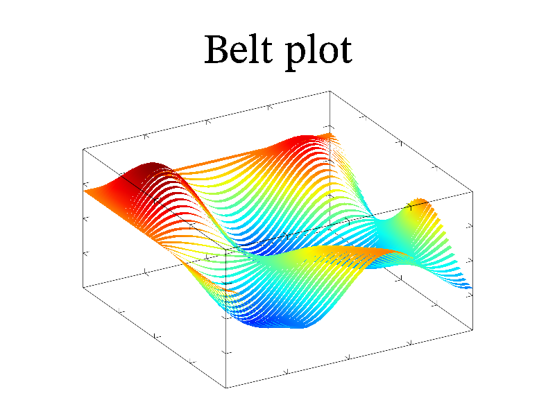
Next: bifurcation sample, Previous: belt sample, Up: All samples [Contents][Index]
Function beltc draw surface by belts. You can use ‘x’ style for drawing lines in other direction.
MGL code:
call 'prepare2d'
title 'BeltC plot':rotate 50 60:box:beltc a b
C++ code:
void smgl_beltc(mglGraph *gr)
{
	mglData a,b;	mgls_prepare2d(&a,&b);
	if(big!=3)	gr->Title("BeltC plot");
	gr->Rotate(50,60);	gr->Box();	gr->BeltC(a,b);
}
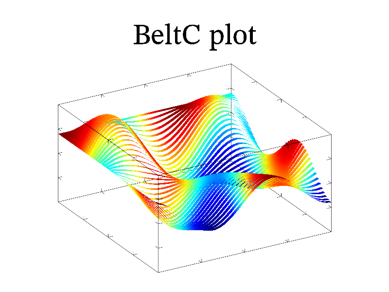
Next: box sample, Previous: beltc sample, Up: All samples [Contents][Index]
Function bifurcation draw Bifurcation diagram for multiple stationary points of the map (like logistic map).
MGL code:
subplot 1 1 0 '<_':title 'Bifurcation sample'
ranges 0 4 0 1:axis
bifurcation 0.005 'x*y*(1-y)' 'r'
C++ code:
void smgl_bifurcation(mglGraph *gr)
{
	gr->SubPlot(1,1,0,"<_");
	if(big!=3)	gr->Title("Bifurcation sample");
	gr->SetRanges(0,4,0,1);	gr->Axis();
	gr->Bifurcation(0.005,"x*y*(1-y)","r");
}

Next: boxplot sample, Previous: bifurcation sample, Up: All samples [Contents][Index]
Different styles of bounding box.
MGL code:
subplot 2 2 0:title 'Box (default)':rotate 50 60:box
subplot 2 2 1:title 'colored':rotate 50 60:box 'r'
subplot 2 2 2:title 'with faces':rotate 50 60:box '@'
subplot 2 2 3:title 'both':rotate 50 60:box '@cm'
C++ code:
void smgl_boxplot(mglGraph *gr)	// flow threads and density plot
{
	mglData a(10,7);	a.Modify("(2*rnd-1)^3/2");
	if(big!=3)	{	gr->SubPlot(1,1,0,"");	gr->Title("Boxplot plot");	}
	gr->Box();	gr->BoxPlot(a);
}
Next: boxs sample, Previous: box sample, Up: All samples [Contents][Index]
Function boxplot draw box-and-whisker diagram.
MGL code:
new a 10 7 '(2*rnd-1)^3/2'
subplot 1 1 0 '':title 'Boxplot plot':box:boxplot a
C++ code:
void smgl_boxplot(mglGraph *gr)	// flow threads and density plot
{
	mglData a(10,7);	a.Modify("(2*rnd-1)^3/2");
	if(big!=3)	{	gr->SubPlot(1,1,0,"");	gr->Title("Boxplot plot");	}
	gr->Box();	gr->BoxPlot(a);
}

Next: candle sample, Previous: boxplot sample, Up: All samples [Contents][Index]
Function boxs draw surface by boxes. You can use ‘#’ for drawing wire plot.
MGL code:
call 'prepare2d'
origin 0 0 0
subplot 2 2 0:title 'Boxs plot (default)':rotate 40 60:light on:box:boxs a
subplot 2 2 1:title '"\@" style':rotate 50 60:box:boxs a '@'
subplot 2 2 2:title '"\#" style':rotate 50 60:box:boxs a '#'
subplot 2 2 3:title 'compare with Tile':rotate 50 60:box:tile a
C++ code:
void smgl_boxs(mglGraph *gr)
{
	mglData a;	mgls_prepare2d(&a);
	gr->SetOrigin(0,0,0);	gr->Light(true);
	if(big!=3)	{gr->SubPlot(2,2,0);	gr->Title("Boxs plot (default)");}
	gr->Rotate(40,60);	gr->Box();	gr->Boxs(a);
	if(big==3)	return;
	gr->SubPlot(2,2,1);	gr->Title("'\\@' style");
	gr->Rotate(50,60);	gr->Box();	gr->Boxs(a,"@");
	gr->SubPlot(2,2,2);	gr->Title("'\\#' style");
	gr->Rotate(50,60);	gr->Box();	gr->Boxs(a,"#");
	gr->SubPlot(2,2,3);	gr->Title("compare with Tile");
	gr->Rotate(50,60);	gr->Box();	gr->Tile(a);
}
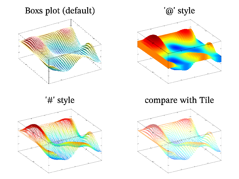
Next: chart sample, Previous: boxs sample, Up: All samples [Contents][Index]
Function candle draw candlestick chart. This is a combination of a line-chart and a bar-chart, in that each bar represents the range of price movement over a given time interval.
MGL code:
new y 30 'sin(pi*x/2)^2'
subplot 1 1 0 '':title 'Candle plot (default)'
yrange 0 1:box
candle y y/2 (y+1)/2
C++ code:
void smgl_candle(mglGraph *gr)
{
	mglData y(30);	gr->Fill(y,"sin(pi*x/2)^2");
	mglData y1(30);	gr->Fill(y1,"v/2",y);
	mglData y2(30);	gr->Fill(y2,"(1+v)/2",y);
	if(big!=3)	{	gr->SubPlot(1,1,0,"");	gr->Title("Candle plot (default)");	}
	gr->SetRange('y',0,1);	gr->Box();	gr->Candle(y,y1,y2);
}

Next: cloud sample, Previous: candle sample, Up: All samples [Contents][Index]
Function chart draw colored boxes with width proportional to data values. Use ‘ ’ for empty box. It produce well known pie chart if drawn in polar coordinates.
MGL code:
new ch 7 2 'rnd+0.1':light on
subplot 2 2 0:title 'Chart plot (default)':rotate 50 60:box:chart ch
subplot 2 2 1:title '"\#" style':rotate 50 60:box:chart ch '#'
subplot 2 2 2:title 'Pie chart; " " color':rotate 50 60:
axis '(y+1)/2*cos(pi*x)' '(y+1)/2*sin(pi*x)' '':box:chart ch 'bgr cmy#'
subplot 2 2 3:title 'Ring chart; " " color':rotate 50 60:
axis '(y+2)/3*cos(pi*x)' '(y+2)/3*sin(pi*x)' '':box:chart ch 'bgr cmy#'
C++ code:
void smgl_chart(mglGraph *gr)
{
	mglData ch(7,2);	for(int i=0;i<7*2;i++)	ch.a[i]=mgl_rnd()+0.1;
	if(big!=3)	{	gr->SubPlot(2,2,0);	gr->Title("Chart plot (default)");	}
	gr->Light(true);	gr->Rotate(50,60);	gr->Box();	gr->Chart(ch);
	if(big==3)	return;
	gr->SubPlot(2,2,1);	gr->Title("'\\#' style");
	gr->Rotate(50,60);	gr->Box();	gr->Chart(ch,"#");
	gr->SubPlot(2,2,2);	gr->Title("Pie chart; ' ' color");
	gr->SetFunc("(y+1)/2*cos(pi*x)","(y+1)/2*sin(pi*x)","");
	gr->Rotate(50,60);	gr->Box();	gr->Chart(ch,"bgr cmy#");
	gr->SubPlot(2,2,3);	gr->Title("Ring chart; ' ' color");
	gr->SetFunc("(y+2)/3*cos(pi*x)","(y+2)/3*sin(pi*x)","");
	gr->Rotate(50,60);	gr->Box();	gr->Chart(ch,"bgr cmy#");
}
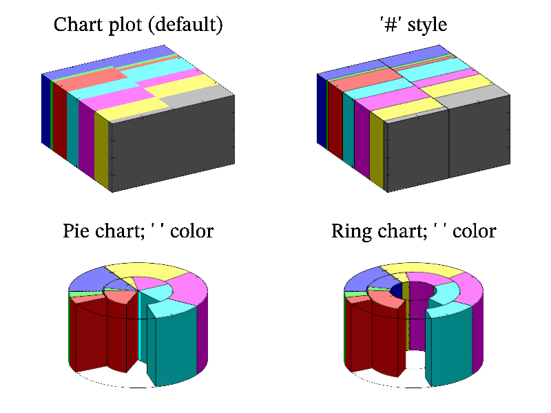
Next: colorbar sample, Previous: chart sample, Up: All samples [Contents][Index]
Function cloud draw cloud-like object which is less transparent for higher data values. Similar plot can be created using many (about 10...20 – surf3a a a;value 10) isosurfaces surf3a.
MGL code:
call 'prepare3d'
subplot 2 2 0:title 'Cloud plot':rotate 50 60:alpha on:box:cloud c 'wyrRk'
subplot 2 2 1:title '"i" style':rotate 50 60:box:cloud c 'iwyrRk'
subplot 2 2 2:title '"." style':rotate 50 60:box:cloud c '.wyrRk'
subplot 2 2 3:title 'meshnum 10':rotate 50 60:box:cloud c 'wyrRk'; meshnum 10
C++ code:
void smgl_cloud(mglGraph *gr)
{
	mglData c;	mgls_prepare3d(&c);
	if(big!=3)	{	gr->SubPlot(2,2,0);	gr->Title("Cloud plot");	}
	gr->Rotate(50,60);	gr->Alpha(true);
	gr->Box();	gr->Cloud(c,"wyrRk");
	if(big==3)	return;
	gr->SubPlot(2,2,1);	gr->Title("'i' style");
	gr->Rotate(50,60);	gr->Box();	gr->Cloud(c,"iwyrRk");
	gr->SubPlot(2,2,2);	gr->Title("'.' style");
	gr->Rotate(50,60);	gr->Box();	gr->Cloud(c,".wyrRk");
	gr->SubPlot(2,2,3);	gr->Title("meshnum 10");
	gr->Rotate(50,60);	gr->Box();	gr->Cloud(c,"wyrRk","meshnum 10");
}
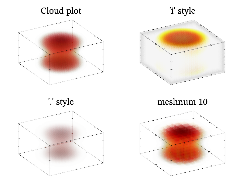
Next: combined sample, Previous: cloud sample, Up: All samples [Contents][Index]
Example of colorbar position and styles.
MGL code:
call 'prepare2d'
new v 9 'x'
subplot 2 2 0:title 'Colorbar out of box':box
colorbar '<':colorbar '>':colorbar '_':colorbar '^'
subplot 2 2 1:title 'Colorbar near box':box
colorbar '<I':colorbar '>I':colorbar '_I':colorbar '^I'
subplot 2 2 2:title 'manual colors':box:contd v a
colorbar v '<':colorbar v '>':colorbar v '_':colorbar v '^'
subplot 2 2 3:title '':text -0.5 1.55 'Color positions' ':C' -2
colorbar 'bwr>' 0.25 0:text -0.9 1.2 'Default'
colorbar 'b{w,0.3}r>' 0.5 0:text -0.1 1.2 'Manual'
crange 0.01 1e3
colorbar '>' 0.75 0:text 0.65 1.2 'Normal scale':colorbar '>':text 1.35 1.2 'Log scale'
C++ code:
void smgl_colorbar(mglGraph *gr)
{
	gr->SubPlot(2,2,0);	gr->Title("Colorbar out of box");	gr->Box();
	gr->Colorbar("<");	gr->Colorbar(">");	gr->Colorbar("_");	gr->Colorbar("^");
	gr->SubPlot(2,2,1);	gr->Title("Colorbar near box");		gr->Box();
	gr->Colorbar("<I");	gr->Colorbar(">I");	gr->Colorbar("_I");	gr->Colorbar("^I");
	gr->SubPlot(2,2,2);	gr->Title("manual colors");
	mglData a,v;	mgls_prepare2d(&a,0,&v);
	gr->Box();	gr->ContD(v,a);
	gr->Colorbar(v,"<");	gr->Colorbar(v,">");	gr->Colorbar(v,"_");	gr->Colorbar(v,"^");

	gr->SubPlot(2,2,3);	gr->Title(" ");
	gr->Puts(mglPoint(-0.5,1.55),"Color positions",":C",-2);
	gr->Colorbar("bwr>",0.25,0);	gr->Puts(mglPoint(-0.9,1.2),"Default");
	gr->Colorbar("b{w,0.3}r>",0.5,0);	gr->Puts(mglPoint(-0.1,1.2),"Manual");

	gr->Puts(mglPoint(1,1.55),"log-scale",":C",-2);
	gr->SetRange('c',0.01,1e3);
	gr->Colorbar(">",0.75,0);	gr->Puts(mglPoint(0.65,1.2),"Normal scale");
	gr->SetFunc("","","","lg(c)");
	gr->Colorbar(">");		gr->Puts(mglPoint(1.35,1.2),"Log scale");
}
Next: cones sample, Previous: colorbar sample, Up: All samples [Contents][Index]
Example of several plots in the same axis.
MGL code:
call 'prepare2v'
call 'prepare3d'
new v 10:fill v -0.5 1:copy d sqrt(a^2+b^2)
subplot 2 2 0:title 'Surf + Cont':rotate 50 60:light on:box:surf a:cont a 'y'
subplot 2 2 1 '':title 'Flow + Dens':light off:box:flow a b 'br':dens d
subplot 2 2 2:title 'Mesh + Cont':rotate 50 60:box:mesh a:cont a '_'
subplot 2 2 3:title 'Surf3 + ContF3':rotate 50 60:light on
box:contf3 v c 'z' 0:contf3 v c 'x':contf3 v c
cut 0 -1 -1 1 0 1.1
contf3 v c 'z' c.nz-1:surf3 c -0.5
C++ code:
void smgl_combined(mglGraph *gr)	// flow threads and density plot
{
	mglData a,b,d;	mgls_prepare2v(&a,&b);	d = a;
	for(int i=0;i<a.nx*a.ny;i++)	d.a[i] = hypot(a.a[i],b.a[i]);
	mglData c;	mgls_prepare3d(&c);
	mglData v(10);	v.Fill(-0.5,1);
	gr->SubPlot(2,2,1,"");	gr->Title("Flow + Dens");
	gr->Flow(a,b,"br");	gr->Dens(d);	gr->Box();
	gr->SubPlot(2,2,0);	gr->Title("Surf + Cont");	gr->Rotate(50,60);
	gr->Light(true);	gr->Surf(a);	gr->Cont(a,"y");	gr->Box();
	gr->SubPlot(2,2,2);	gr->Title("Mesh + Cont");	gr->Rotate(50,60);
	gr->Box();	gr->Mesh(a);	gr->Cont(a,"_");
	gr->SubPlot(2,2,3);	gr->Title("Surf3 + ContF3");gr->Rotate(50,60);
	gr->Box();	gr->ContF3(v,c,"z",0);	gr->ContF3(v,c,"x");	gr->ContF3(v,c);
	gr->SetCutBox(mglPoint(0,-1,-1), mglPoint(1,0,1.1));
	gr->ContF3(v,c,"z",c.nz-1);	gr->Surf3(-0.5,c);
}
Next: cont sample, Previous: combined sample, Up: All samples [Contents][Index]
Function cones is similar to bars but draw cones.
MGL code:
new ys 10 3 '0.8*sin(pi*(x+y/4+1.25))+0.2*rnd'
light on:origin 0 0 0
subplot 3 2 0:title 'Cones plot':rotate 50 60:box:cones ys
subplot 3 2 1:title '2 colors':rotate 50 60:box:cones ys 'cbgGyr'
subplot 3 2 2:title '"\#" style':rotate 50 60:box:cones ys '#'
subplot 3 2 3:title '"a" style':rotate 50 60:zrange -2 2:box:cones ys 'a'
subplot 3 2 4:title '"t" style':rotate 50 60:box:cones ys 't'
subplot 3 2 5:title '"4" style':rotate 50 60:box:cones ys '4'
C++ code:
void smgl_cones(mglGraph *gr)
{
	mglData ys(10,3);	ys.Modify("0.8*sin(pi*(2*x+y/2))+0.2*rnd");
	gr->Light(true);	gr->SetOrigin(0,0,0);
	if(big!=3)	{	gr->SubPlot(3,2,0);	gr->Title("Cones plot");	}
	gr->Rotate(50,60);	gr->Box();	gr->Cones(ys);
	if(big==3)	return;
	gr->SubPlot(3,2,1);	gr->Title("2 colors");
	gr->Rotate(50,60);	gr->Box();	gr->Cones(ys,"cbgGyr");
	gr->SubPlot(3,2,2);	gr->Title("'\\#' style");
	gr->Rotate(50,60);	gr->Box();	gr->Cones(ys,"#");
	gr->SubPlot(3,2,3);	gr->Title("'a' style");
	gr->SetRange('z',-2,2);	// increase range since summation can exceed [-1,1]
	gr->Rotate(50,60);	gr->Box();	gr->Cones(ys,"a");
	gr->SubPlot(3,2,4);	gr->Title("'t' style");
	gr->Rotate(50,60);	gr->Box();	gr->Cones(ys,"t");
	gr->SubPlot(3,2,5);	gr->Title("'4' style");
	gr->Rotate(50,60);	gr->Box();	gr->Cones(ys,"4");
}
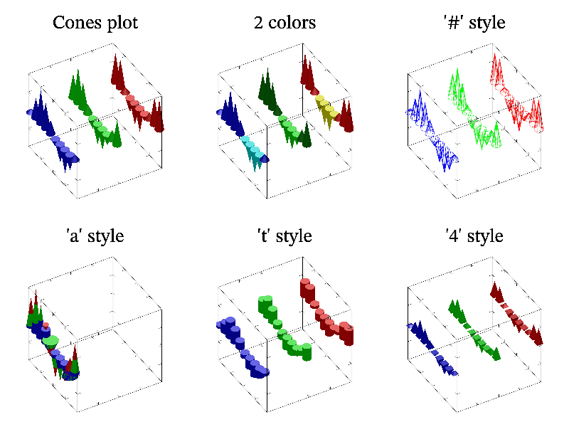
Next: cont3 sample, Previous: cones sample, Up: All samples [Contents][Index]
Function cont draw contour lines for surface. You can select automatic (default) or manual levels for contours, print contour labels, draw it on the surface (default) or at plane (as Dens).
MGL code:
call 'prepare2d'
list v -0.5 -0.15 0 0.15 0.5
subplot 2 2 0:title 'Cont plot (default)':rotate 50 60:box:cont a
subplot 2 2 1:title 'manual levels':rotate 50 60:box:cont v a
subplot 2 2 2:title '"\_" and "." styles':rotate 50 60:box:cont a '_':cont a '_.2k'
subplot 2 2 3 '':title '"t" style':box:cont a 't'
C++ code:
void smgl_cont3(mglGraph *gr)
{
	mglData c;	mgls_prepare3d(&c);
	if(big!=3)	gr->Title("Cont3 sample");
	gr->Rotate(50,60);	gr->Box();
	gr->Cont3(c,"x");	gr->Cont3(c);	gr->Cont3(c,"z");
}
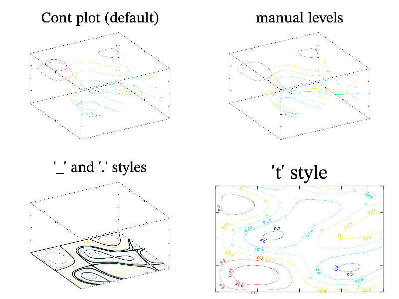
Next: cont_xyz sample, Previous: cont sample, Up: All samples [Contents][Index]
Function contf3 draw ordinary contour lines but at slices of 3D data.
MGL code:
call 'prepare3d'
title 'Cont3 sample':rotate 50 60:box
cont3 c 'x':cont3 c:cont3 c 'z'
C++ code:
void smgl_cont3(mglGraph *gr)
{
	mglData c;	mgls_prepare3d(&c);
	if(big!=3)	gr->Title("Cont3 sample");
	gr->Rotate(50,60);	gr->Box();
	gr->Cont3(c,"x");	gr->Cont3(c);	gr->Cont3(c,"z");
}

Next: contd sample, Previous: cont3 sample, Up: All samples [Contents][Index]
Functions contz, conty, contx draw contour lines on plane perpendicular to corresponding axis. One of possible application is drawing projections of 3D field.
MGL code:
call 'prepare3d'
title 'Cont[XYZ] sample':rotate 50 60:box
contx {sum c 'x'} '' -1:conty {sum c 'y'} '' 1:contz {sum c 'z'} '' -1
C++ code:
void smgl_cont_xyz(mglGraph *gr)
{
	mglData c;	mgls_prepare3d(&c);
	if(big!=3)	gr->Title("Cont[XYZ] sample");
	gr->Rotate(50,60);	gr->Box();	gr->ContX(c.Sum("x"),"",-1);
	gr->ContY(c.Sum("y"),"",1);		gr->ContZ(c.Sum("z"),"",-1);
}
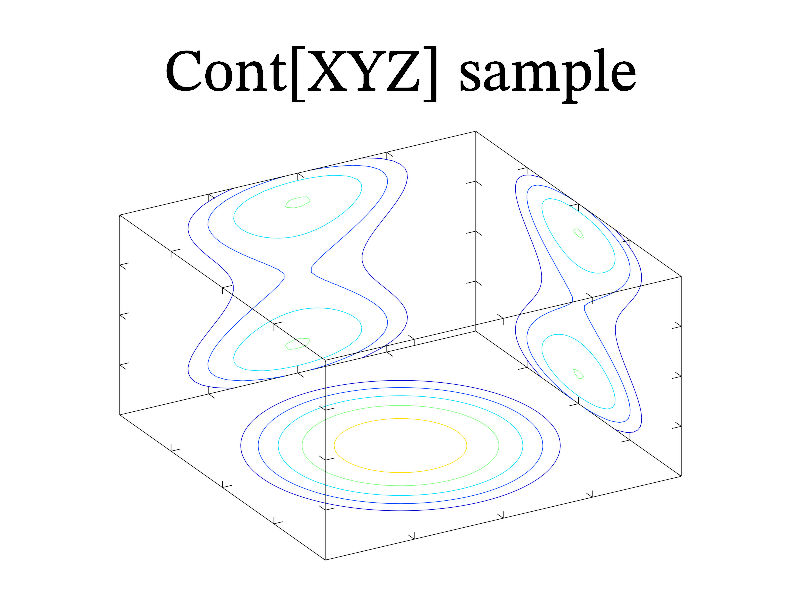
Next: contf sample, Previous: cont_xyz sample, Up: All samples [Contents][Index]
Function contd is similar to contf but with manual contour colors.
MGL code:
call 'prepare2d'
list v -0.5 -0.15 0 0.15 0.5
new a1 30 40 3 '0.6*sin(2*pi*x+pi*(z+1)/2)*sin(3*pi*y+pi*z) + 0.4*cos(3*pi*(x*y)+pi*(z+1)^2/2)'
subplot 2 2 0:title 'ContD plot (default)':rotate 50 60:box:contd a
subplot 2 2 1:title 'manual levels':rotate 50 60:box:contd v a
subplot 2 2 2:title '"\_" style':rotate 50 60:box:contd a '_'
subplot 2 2 3:title 'several slices':rotate 50 60:box:contd a1
C++ code:
void smgl_contd(mglGraph *gr)
{
	mglData a,v(5),a1(30,40,3);	mgls_prepare2d(&a);	v.a[0]=-0.5;
	v.a[1]=-0.15;	v.a[2]=0;	v.a[3]=0.15;	v.a[4]=0.5;
	gr->Fill(a1,"0.6*sin(2*pi*x+pi*(z+1)/2)*sin(3*pi*y+pi*z) + 0.4*cos(3*pi*(x*y)+pi*(z+1)^2/2)");

	if(big!=3)	{	gr->SubPlot(2,2,0);	gr->Title("ContD plot (default)");	}
	gr->Rotate(50,60);	gr->Box();	gr->ContD(a);
	if(big==3)	return;
	gr->SubPlot(2,2,1);	gr->Title("manual levels");
	gr->Rotate(50,60);	gr->Box();	gr->ContD(v,a);
	gr->SubPlot(2,2,2);	gr->Title("'\\_' style");
	gr->Rotate(50,60);	gr->Box();	gr->ContD(a,"_");
	gr->SubPlot(2,2,3);	gr->Title("several slices");
	gr->Rotate(50,60);	gr->Box();	gr->ContD(a1);
}
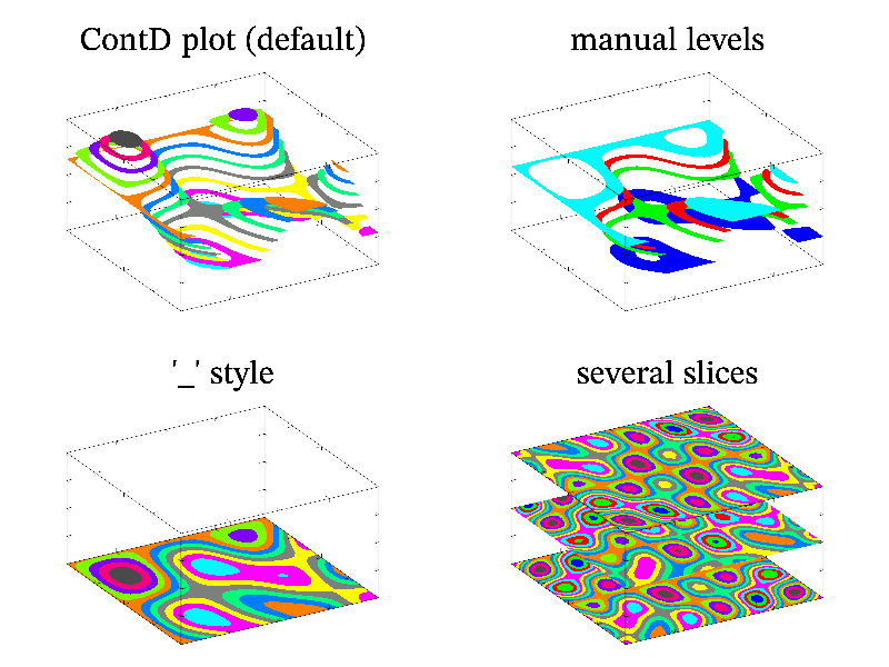
Next: contf3 sample, Previous: contd sample, Up: All samples [Contents][Index]
Function contf draw filled contours. You can select automatic (default) or manual levels for contours.
MGL code:
call 'prepare2d'
list v -0.5 -0.15 0 0.15 0.5
new a1 30 40 3 '0.6*sin(2*pi*x+pi*(z+1)/2)*sin(3*pi*y+pi*z) + 0.4*cos(3*pi*(x*y)+pi*(z+1)^2/2)'
subplot 2 2 0:title 'ContF plot (default)':rotate 50 60:box:contf a
subplot 2 2 1:title 'manual levels':rotate 50 60:box:contf v a
subplot 2 2 2:title '"\_" style':rotate 50 60:box:contf a '_'
subplot 2 2 3:title 'several slices':rotate 50 60:box:contf a1
C++ code:
void smgl_contf3(mglGraph *gr)
{
mglData c; mgls_prepare3d(&c);
if(big!=3) gr->Title("ContF3 sample");
gr->Rotate(50,60); gr->Light(true); gr->Box();
gr->ContF3(c,"x"); gr->ContF3(c); gr->ContF3(c,"z");
gr->Cont3(c,"kx"); gr->Cont3(c,"k"); gr->Cont3(c,"kz");
}
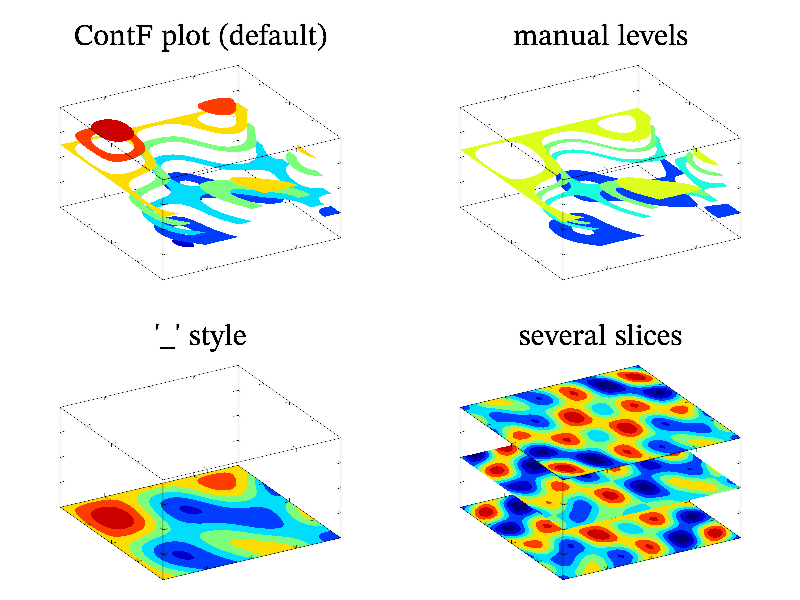
Next: contf_xyz sample, Previous: contf sample, Up: All samples [Contents][Index]
Function contf3 draw ordinary filled contours but at slices of 3D data.
MGL code:
call 'prepare3d' title 'Cont3 sample':rotate 50 60:box:light on contf3 c 'x':contf3 c:contf3 c 'z' cont3 c 'xk':cont3 c 'k':cont3 c 'zk'
C++ code:
void smgl_contf3(mglGraph *gr)
{
mglData c; mgls_prepare3d(&c);
if(big!=3) gr->Title("ContF3 sample");
gr->Rotate(50,60); gr->Light(true); gr->Box();
gr->ContF3(c,"x"); gr->ContF3(c); gr->ContF3(c,"z");
gr->Cont3(c,"kx"); gr->Cont3(c,"k"); gr->Cont3(c,"kz");
}

Next: conts sample, Previous: contf3 sample, Up: All samples [Contents][Index]
Functions contfz, contfy, contfx, draw filled contours on plane perpendicular to corresponding axis. One of possible application is drawing projections of 3D field.
MGL code:
call 'prepare3d'
title 'ContF[XYZ] sample':rotate 50 60:box
contfx {sum c 'x'} '' -1:contfy {sum c 'y'} '' 1:contfz {sum c 'z'} '' -1
C++ code:
void smgl_contf_xyz(mglGraph *gr)
{
mglData c; mgls_prepare3d(&c);
if(big!=3) gr->Title("ContF[XYZ] sample");
gr->Rotate(50,60); gr->Box(); gr->ContFX(c.Sum("x"),"",-1);
gr->ContFY(c.Sum("y"),"",1); gr->ContFZ(c.Sum("z"),"",-1);
}
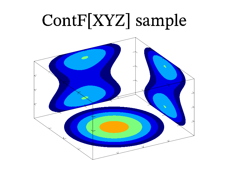
Next: contv sample, Previous: contf_xyz sample, Up: All samples [Contents][Index]
Function conts get contour coordinate as data array.
MGL code:
new a 10 10 'sin(2*pi*x*y)' title 'Conts sample':rotate 40 60:box dens a '#' cont [0,0] a 'r' conts r 0 a plot 2*r(0)-1 2*r(1)-1 1+r(2) '2c'
C++ code:
void smgl_conts(mglGraph *gr) // test conts
{
mglData a(10,10); gr->Fill(a,"sin(2*pi*x*y)");
mglData v, r=a.Conts(0);
if(big!=3) { gr->Title("Conts sample"); }
gr->Rotate(40,60); gr->Box();
gr->Dens(a,"#"); gr->Cont(v,a,"r");
mglData x(r.ny),y(r.ny),z(r.ny);
for(long i=0;i<x.nx;i++) { x[i]=r[r.nx*i]*2-1; y[i]=r[r.nx*i+1]*2-1; z[i]=1; }
gr->Plot(x,y,z,"2c");
}
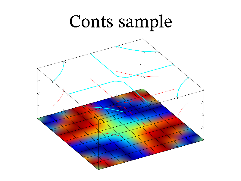
Next: correl sample, Previous: conts sample, Up: All samples [Contents][Index]
Function contv draw vertical cylinders (belts) at contour lines.
MGL code:
call 'prepare2d' list v -0.5 -0.15 0 0.15 0.5 subplot 2 2 0:title 'ContV plot (default)':rotate 50 60:box:contv a subplot 2 2 1:title 'manual levels':rotate 50 60:box:contv v a subplot 2 2 2:title '"\_" style':rotate 50 60:box:contv a '_' subplot 2 2 3:title 'ContV and ContF':rotate 50 60:light on:box contv a:contf a:cont a 'k'
C++ code:
void smgl_contv(mglGraph *gr)
{
mglData a,v(5); mgls_prepare2d(&a); v.a[0]=-0.5;
v.a[1]=-0.15; v.a[2]=0; v.a[3]=0.15; v.a[4]=0.5;
if(big!=3) { gr->SubPlot(2,2,0); gr->Title("ContV plot (default)"); }
gr->Rotate(50,60); gr->Box(); gr->ContV(a);
if(big==3) return;
gr->SubPlot(2,2,1); gr->Title("manual levels");
gr->Rotate(50,60); gr->Box(); gr->ContV(v,a);
gr->SubPlot(2,2,2); gr->Title("'\\_' style");
gr->Rotate(50,60); gr->Box(); gr->ContV(a,"_");
gr->SubPlot(2,2,3); gr->Title("ContV and ContF");
gr->Rotate(50,60); gr->Box(); gr->Light(true);
gr->ContV(a); gr->ContF(a); gr->Cont(a,"k");
}
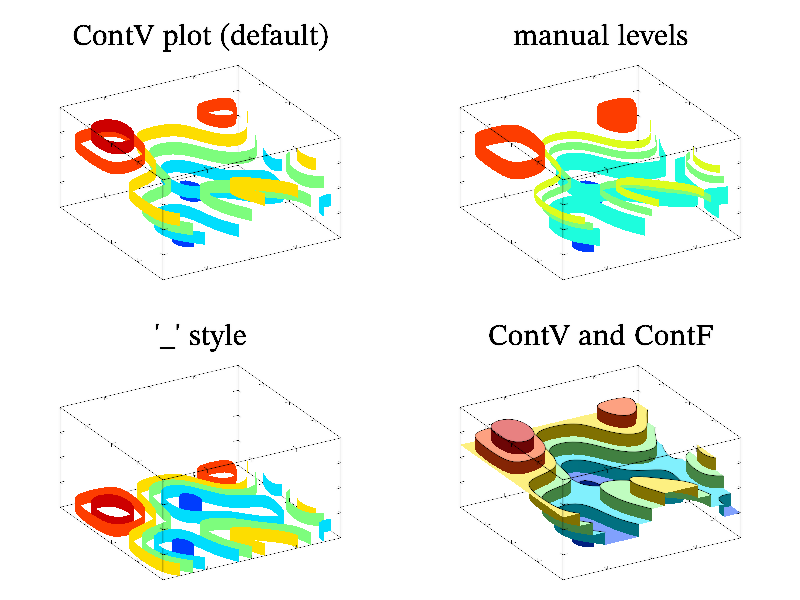
Next: curvcoor sample, Previous: contv sample, Up: All samples [Contents][Index]
Test of correlation function (correl).
MGL code:
new a 100 'exp(-10*x^2)' new b 100 'exp(-10*(x+0.5)^2)' yrange 0 1 subplot 1 2 0 '_':title 'Input fields' plot a:plot b:box:axis correl r a b 'x' norm r 0 1:swap r 'x' # make it human readable subplot 1 2 1 '_':title 'Correlation of a and b' plot r 'r':axis:box line 0.5 0 0.5 1 'B|'
C++ code:
void smgl_correl(mglGraph *gr)
{
mglData a(100),b(100);
gr->Fill(a,"exp(-10*x^2)"); gr->Fill(b,"exp(-10*(x+0.5)^2)");
gr->SetRange('y',0,1);
gr->SubPlot(1,2,0,"_"); gr->Title("Input fields");
gr->Plot(a); gr->Plot(b); gr->Axis(); gr->Box();
mglData r = a.Correl(b,"x");
r.Norm(0,1); r.Swap("x"); // make it human readable
gr->SubPlot(1,2,1,"_"); gr->Title("Correlation of a and b");
gr->Plot(r,"r"); gr->Axis(); gr->Box();
gr->Line(mglPoint(0.5,0),mglPoint(0.5,1),"B|");
}
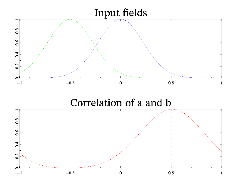
Next: cut sample, Previous: correl sample, Up: All samples [Contents][Index]
Some common curvilinear coordinates.
MGL code:
origin -1 1 -1 subplot 2 2 0:title 'Cartesian':rotate 50 60:fplot '2*t-1' '0.5' '0' '2r':axis:grid axis 'y*sin(pi*x)' 'y*cos(pi*x)' '':subplot 2 2 1:title 'Cylindrical':rotate 50 60:fplot '2*t-1' '0.5' '0' '2r':axis:grid axis '2*y*x' 'y*y - x*x' '':subplot 2 2 2:title 'Parabolic':rotate 50 60:fplot '2*t-1' '0.5' '0' '2r':axis:grid axis 'y*sin(pi*x)' 'y*cos(pi*x)' 'x+z':subplot 2 2 3:title 'Spiral':rotate 50 60:fplot '2*t-1' '0.5' '0' '2r':axis:grid
C++ code:
void smgl_curvcoor(mglGraph *gr) // curvilinear coordinates
{
gr->SetOrigin(-1,1,-1);
gr->SubPlot(2,2,0); gr->Title("Cartesian"); gr->Rotate(50,60);
gr->FPlot("2*t-1","0.5","0","r2");
gr->Axis(); gr->Grid();
gr->SetFunc("y*sin(pi*x)","y*cos(pi*x)",0);
gr->SubPlot(2,2,1); gr->Title("Cylindrical"); gr->Rotate(50,60);
gr->FPlot("2*t-1","0.5","0","r2");
gr->Axis(); gr->Grid();
gr->SetFunc("2*y*x","y*y - x*x",0);
gr->SubPlot(2,2,2); gr->Title("Parabolic"); gr->Rotate(50,60);
gr->FPlot("2*t-1","0.5","0","r2");
gr->Axis(); gr->Grid();
gr->SetFunc("y*sin(pi*x)","y*cos(pi*x)","x+z");
gr->SubPlot(2,2,3); gr->Title("Spiral"); gr->Rotate(50,60);
gr->FPlot("2*t-1","0.5","0","r2");
gr->Axis(); gr->Grid();
gr->SetFunc(0,0,0); // set to default Cartesian
}
Next: daisy sample, Previous: curvcoor sample, Up: All samples [Contents][Index]
Example of point cutting (cut.
MGL code:
call 'prepare2d' call 'prepare3d' subplot 2 2 0:title 'Cut on (default)':rotate 50 60:light on:box:surf a; zrange -1 0.5 subplot 2 2 1:title 'Cut off':rotate 50 60:box:surf a; zrange -1 0.5; cut off subplot 2 2 2:title 'Cut in box':rotate 50 60:box:alpha on cut 0 -1 -1 1 0 1.1:surf3 c cut 0 0 0 0 0 0 # restore back subplot 2 2 3:title 'Cut by formula':rotate 50 60:box cut '(z>(x+0.5*y-1)^2-1) & (z>(x-0.5*y-1)^2-1)':surf3 c
C++ code:
void smgl_cut(mglGraph *gr) // cutting
{
mglData a,c,v(1); mgls_prepare2d(&a); mgls_prepare3d(&c); v.a[0]=0.5;
gr->SubPlot(2,2,0); gr->Title("Cut on (default)"); gr->Rotate(50,60); gr->Light(true);
gr->Box(); gr->Surf(a,"","zrange -1 0.5");
gr->SubPlot(2,2,1); gr->Title("Cut off"); gr->Rotate(50,60);
gr->Box(); gr->Surf(a,"","zrange -1 0.5; cut off");
gr->SubPlot(2,2,2); gr->Title("Cut in box"); gr->Rotate(50,60);
gr->SetCutBox(mglPoint(0,-1,-1), mglPoint(1,0,1.1));
gr->Alpha(true); gr->Box(); gr->Surf3(c);
gr->SetCutBox(mglPoint(0), mglPoint(0)); // switch it off
gr->SubPlot(2,2,3); gr->Title("Cut by formula"); gr->Rotate(50,60);
gr->CutOff("(z>(x+0.5*y-1)^2-1) & (z>(x-0.5*y-1)^2-1)");
gr->Box(); gr->Surf3(c); gr->CutOff(""); // switch it off
}
Next: dat_diff sample, Previous: cut sample, Up: All samples [Contents][Index]
Example of subfunctions and summation in textual formulas.
MGL code:
title 'Advanced formulas' new b 256 256 'dsum(fn1(_i*pi/5),10)\exp(-64*(x*cos(_1)-y*sin(_1))^2-16*(0.5+y*cos(_1)+x*sin(_1))^2)' crange b:dens b 'BbwrR'
C++ code:
void smgl_daisy(mglGraph *gr)
{
if(big!=3) gr->Title("Advanced formulas");
mglData b(256,256);
gr->Fill(b,"dsum(fn1(_i*pi/5),10)\\exp(-64*(x*cos(_1)-y*sin(_1))^2-16*(0.5+y*cos(_1)+x*sin(_1))^2)");
gr->SetRange('c',b); gr->Dens(b,"BbwrR");
}
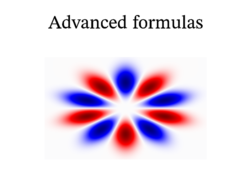
Next: dat_extra sample, Previous: daisy sample, Up: All samples [Contents][Index]
Example of diff and integrate.
MGL code:
ranges 0 1 0 1 0 1:new a 30 40 'x*y'
subplot 2 2 0:title 'a(x,y)':rotate 60 40:surf a:box
subplot 2 2 1:title 'da/dx':rotate 60 40:diff a 'x':surf a:box
subplot 2 2 2:title '\int da/dx dxdy':rotate 60 40:integrate a 'xy':surf a:box
subplot 2 2 3:title '\int {d^2}a/dxdy dx':rotate 60 40:diff2 a 'y':surf a:box
C++ code:
void smgl_dat_diff(mglGraph *gr) // differentiate
{
gr->SetRanges(0,1,0,1,0,1);
mglData a(30,40); a.Modify("x*y");
gr->SubPlot(2,2,0); gr->Title("a(x,y)"); gr->Rotate(60,40);
gr->Surf(a); gr->Box();
gr->SubPlot(2,2,1); gr->Title("da/dx"); gr->Rotate(60,40);
a.Diff("x"); gr->Surf(a); gr->Box();
gr->SubPlot(2,2,2); gr->Title("\\int da/dx dxdy"); gr->Rotate(60,40);
a.Integral("xy"); gr->Surf(a); gr->Box();
gr->SubPlot(2,2,3); gr->Title("\\int {d^2}a/dxdy dx"); gr->Rotate(60,40);
a.Diff2("y"); gr->Surf(a); gr->Box();
}
Next: data1 sample, Previous: dat_diff sample, Up: All samples [Contents][Index]
Example of envelop, sew, smooth and resize.
MGL code:
subplot 2 2 0 '':title 'Envelop sample':new d1 1000 'exp(-8*x^2)*sin(10*pi*x)'
axis:plot d1 'b':envelop d1 'x':plot d1 'r'
subplot 2 2 1 '':title 'Smooth sample':ranges 0 1 0 1
new y0 30 '0.4*sin(pi*x) + 0.3*cos(1.5*pi*x) - 0.4*sin(2*pi*x)+0.5*rnd'
copy y1 y0:smooth y1 'x3':plot y1 'r';legend '"3" style'
copy y2 y0:smooth y2 'x5':plot y2 'g';legend '"5" style'
copy y3 y0:smooth y3 'x':plot y3 'b';legend 'default'
plot y0 '{m7}:s';legend 'none'
legend:box
subplot 2 2 2:title 'Sew sample':rotate 50 60:light on:alpha on
new d2 100 100 'mod((y^2-(1-x)^2)/2,0.1)'
box:surf d2 'b':sew d2 'xy' 0.1:surf d2 'r'
subplot 2 2 3:title 'Resize sample (interpolation)'
new x0 10 'rnd':new v0 10 'rnd'
resize x1 x0 100:resize v1 v0 100
plot x0 v0 'b+ ':plot x1 v1 'r-':label x0 v0 '%n'
C++ code:
void smgl_dat_extra(mglGraph *gr) // differentiate
{
gr->SubPlot(2,2,0,""); gr->Title("Envelop sample");
mglData d1(1000); gr->Fill(d1,"exp(-8*x^2)*sin(10*pi*x)");
gr->Axis(); gr->Plot(d1, "b");
d1.Envelop('x'); gr->Plot(d1, "r");
gr->SubPlot(2,2,1,""); gr->Title("Smooth sample");
mglData y0(30),y1,y2,y3;
gr->SetRanges(0,1,0,1);
gr->Fill(y0, "0.4*sin(pi*x) + 0.3*cos(1.5*pi*x) - 0.4*sin(2*pi*x)+0.5*rnd");
y1=y0; y1.Smooth("x3");
y2=y0; y2.Smooth("x5");
y3=y0; y3.Smooth("x");
gr->Plot(y0,"{m7}:s", "legend 'none'"); //gr->AddLegend("none","k");
gr->Plot(y1,"r", "legend ''3' style'");
gr->Plot(y2,"g", "legend ''5' style'");
gr->Plot(y3,"b", "legend 'default'");
gr->Legend(); gr->Box();
gr->SubPlot(2,2,2); gr->Title("Sew sample");
mglData d2(100, 100); gr->Fill(d2, "mod((y^2-(1-x)^2)/2,0.1)");
gr->Rotate(50, 60); gr->Light(true); gr->Alpha(true);
gr->Box(); gr->Surf(d2, "b");
d2.Sew("xy", 0.1); gr->Surf(d2, "r");
gr->SubPlot(2,2,3); gr->Title("Resize sample (interpolation)");
mglData x0(10), v0(10), x1, v1;
gr->Fill(x0,"rnd"); gr->Fill(v0,"rnd");
x1 = x0.Resize(100); v1 = v0.Resize(100);
gr->Plot(x0,v0,"b+ "); gr->Plot(x1,v1,"r-");
gr->Label(x0,v0,"%n");
}
Next: data2 sample, Previous: dat_extra sample, Up: All samples [Contents][Index]
MGL code:
new a 40 50 60 'exp(-x^2-4*y^2-16*z^2)' light on:alpha on copy b a:diff b 'x':subplot 5 3 0:call 'splot' copy b a:diff2 b 'x':subplot 5 3 1:call 'splot' copy b a:cumsum b 'x':subplot 5 3 2:call 'splot' copy b a:integrate b 'x':subplot 5 3 3:call 'splot' mirror b 'x':subplot 5 3 4:call 'splot' copy b a:diff b 'y':subplot 5 3 5:call 'splot' copy b a:diff2 b 'y':subplot 5 3 6:call 'splot' copy b a:cumsum b 'y':subplot 5 3 7:call 'splot' copy b a:integrate b 'y':subplot 5 3 8:call 'splot' mirror b 'y':subplot 5 3 9:call 'splot' copy b a:diff b 'z':subplot 5 3 10:call 'splot' copy b a:diff2 b 'z':subplot 5 3 11:call 'splot' copy b a:cumsum b 'z':subplot 5 3 12:call 'splot' copy b a:integrate b 'z':subplot 5 3 13:call 'splot' mirror b 'z':subplot 5 3 14:call 'splot' stop func splot 0 title 'max=',b.max:norm b -1 1 on:rotate 70 60:box:surf3 b return
C++ code:
void smgl_data1(mglGraph *gr) // basic data operations
{
mglData a(40,50,60),b; gr->Fill(a,"exp(-x^2-4*y^2-16*z^2)");
gr->Light(true); gr->Alpha(true);
b.Set(a); b.Diff("x"); gr->SubPlot(5,3,0); splot1(gr,b);
b.Set(a); b.Diff2("x"); gr->SubPlot(5,3,1); splot1(gr,b);
b.Set(a); b.CumSum("x"); gr->SubPlot(5,3,2); splot1(gr,b);
b.Set(a); b.Integral("x");gr->SubPlot(5,3,3); splot1(gr,b);
b.Mirror("x"); gr->SubPlot(5,3,4); splot1(gr,b);
b.Set(a); b.Diff("y"); gr->SubPlot(5,3,5); splot1(gr,b);
b.Set(a); b.Diff2("y"); gr->SubPlot(5,3,6); splot1(gr,b);
b.Set(a); b.CumSum("y"); gr->SubPlot(5,3,7); splot1(gr,b);
b.Set(a); b.Integral("y");gr->SubPlot(5,3,8); splot1(gr,b);
b.Mirror("y"); gr->SubPlot(5,3,9); splot1(gr,b);
b.Set(a); b.Diff("z"); gr->SubPlot(5,3,10);splot1(gr,b);
b.Set(a); b.Diff2("z"); gr->SubPlot(5,3,11);splot1(gr,b);
b.Set(a); b.CumSum("z"); gr->SubPlot(5,3,12);splot1(gr,b);
b.Set(a); b.Integral("z");gr->SubPlot(5,3,13);splot1(gr,b);
b.Mirror("z"); gr->SubPlot(5,3,14);splot1(gr,b);
}
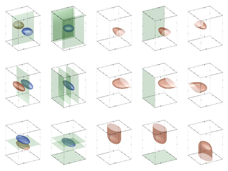
Next: dcont sample, Previous: data1 sample, Up: All samples [Contents][Index]
MGL code:
new a 40 50 60 'exp(-x^2-4*y^2-16*z^2)' light on:alpha on copy b a:sinfft b 'x':subplot 5 3 0:call 'splot' copy b a:cosfft b 'x':subplot 5 3 1:call 'splot' copy b a:hankel b 'x':subplot 5 3 2:call 'splot' copy b a:swap b 'x':subplot 5 3 3:call 'splot' copy b a:smooth b 'x':subplot 5 3 4:call 'splot' copy b a:sinfft b 'y':subplot 5 3 5:call 'splot' copy b a:cosfft b 'y':subplot 5 3 6:call 'splot' copy b a:hankel b 'y':subplot 5 3 7:call 'splot' copy b a:swap b 'y':subplot 5 3 8:call 'splot' copy b a:smooth b 'y':subplot 5 3 9:call 'splot' copy b a:sinfft b 'z':subplot 5 3 10:call 'splot' copy b a:cosfft b 'z':subplot 5 3 11:call 'splot' copy b a:hankel b 'z':subplot 5 3 12:call 'splot' copy b a:swap b 'z':subplot 5 3 13:call 'splot' copy b a:smooth b 'z':subplot 5 3 14:call 'splot' stop func splot 0 title 'max=',b.max:norm b -1 1 on:rotate 70 60:box surf3 b 0.5:surf3 b -0.5 return
C++ code:
void smgl_data2(mglGraph *gr) // data transforms
{
mglData a(40,50,60),b; gr->Fill(a,"exp(-x^2-4*y^2-16*z^2)");
gr->Light(true); gr->Alpha(true);
b.Set(a); b.SinFFT("x"); gr->SubPlot(5,3,0); splot2(gr,b);
b.Set(a); b.CosFFT("x"); gr->SubPlot(5,3,1); splot2(gr,b);
b.Set(a); b.Hankel("x"); gr->SubPlot(5,3,2); splot2(gr,b);
b.Set(a); b.Swap("x"); gr->SubPlot(5,3,3); splot2(gr,b);
b.Set(a); b.Smooth("x"); gr->SubPlot(5,3,4); splot2(gr,b);
b.Set(a); b.SinFFT("y"); gr->SubPlot(5,3,5); splot2(gr,b);
b.Set(a); b.CosFFT("y"); gr->SubPlot(5,3,6); splot2(gr,b);
b.Set(a); b.Hankel("y"); gr->SubPlot(5,3,7); splot2(gr,b);
b.Set(a); b.Swap("y"); gr->SubPlot(5,3,8); splot2(gr,b);
b.Set(a); b.Smooth("y"); gr->SubPlot(5,3,9); splot2(gr,b);
b.Set(a); b.SinFFT("z"); gr->SubPlot(5,3,10);splot2(gr,b);
b.Set(a); b.CosFFT("z"); gr->SubPlot(5,3,11);splot2(gr,b);
b.Set(a); b.Hankel("z"); gr->SubPlot(5,3,12);splot2(gr,b);
b.Set(a); b.Swap("z"); gr->SubPlot(5,3,13);splot2(gr,b);
b.Set(a); b.Smooth("z"); gr->SubPlot(5,3,14);splot2(gr,b);
}
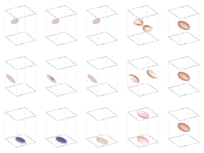
Next: dens sample, Previous: data2 sample, Up: All samples [Contents][Index]
Function dcont draw lines of intersections of two isosurfaces.
MGL code:
call 'prepare3d' title 'DCont plot':rotate 50 60:light on:alpha on:box:surf3 c 0 'r':surf3 d 0 'b' dcont 0 c d '2k'
C++ code:
void smgl_dcont(mglGraph *gr)
{
mglData c,d,v; mgls_prepare3d(&c,&d);
if(big!=3) gr->Title("DCont plot");
gr->Rotate(50,60); gr->Light(true); gr->Alpha(true);
gr->Box(); gr->Surf3(0,c,"r"); gr->Surf3(0,d,"b");
gr->DCont(v,c,d,"2k");
}
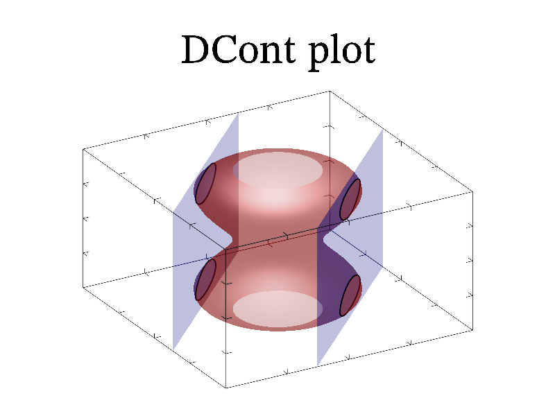
Next: dens3 sample, Previous: dcont sample, Up: All samples [Contents][Index]
Function dens draw density plot (also known as color-map) for surface.
MGL code:
call 'prepare2d' new a1 30 40 3 '0.6*sin(2*pi*x+pi*(z+1)/2)*sin(3*pi*y+pi*z) + 0.4*cos(3*pi*(x*y)+pi*(z+1)^2/2)' subplot 2 2 0 '':title 'Dens plot (default)':box:dens a subplot 2 2 1:title '3d variant':rotate 50 60:box:dens a subplot 2 2 2 '':title '"\#" style; meshnum 10':box:dens a '#'; meshnum 10 subplot 2 2 3:title 'several slices':rotate 50 60:box:dens a1
C++ code:
void smgl_dens3(mglGraph *gr)
{
mglData c; mgls_prepare3d(&c);
if(big!=3) gr->Title("Dens3 sample");
gr->Rotate(50,60); gr->Alpha(true); gr->SetAlphaDef(0.7);
gr->SetOrigin(0,0,0); gr->Axis("_xyz"); gr->Box();
gr->Dens3(c,"x"); gr->Dens3(c); gr->Dens3(c,"z");
}
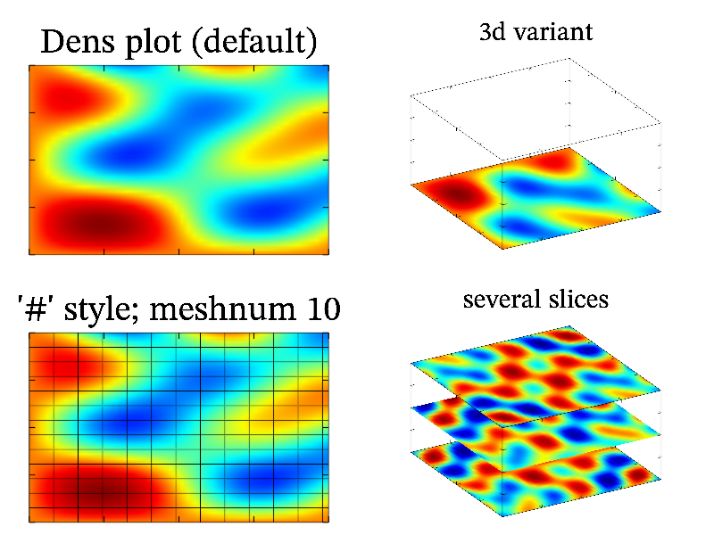
Next: dens_xyz sample, Previous: dens sample, Up: All samples [Contents][Index]
Function dens3 draw ordinary density plots but at slices of 3D data.
MGL code:
call 'prepare3d' title 'Dens3 sample':rotate 50 60:alpha on:alphadef 0.7 origin 0 0 0:box:axis '_xyz' dens3 c 'x':dens3 c ':y':dens3 c 'z'
C++ code:
void smgl_dens3(mglGraph *gr)
{
mglData c; mgls_prepare3d(&c);
if(big!=3) gr->Title("Dens3 sample");
gr->Rotate(50,60); gr->Alpha(true); gr->SetAlphaDef(0.7);
gr->SetOrigin(0,0,0); gr->Axis("_xyz"); gr->Box();
gr->Dens3(c,"x"); gr->Dens3(c); gr->Dens3(c,"z");
}
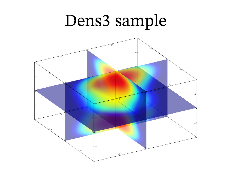
Next: detect sample, Previous: dens3 sample, Up: All samples [Contents][Index]
Functions densz, densy, densx draw density plot on plane perpendicular to corresponding axis. One of possible application is drawing projections of 3D field.
MGL code:
call 'prepare3d'
title 'Dens[XYZ] sample':rotate 50 60:box
densx {sum c 'x'} '' -1:densy {sum c 'y'} '' 1:densz {sum c 'z'} '' -1
C++ code:
void smgl_dens_xyz(mglGraph *gr)
{
mglData c; mgls_prepare3d(&c);
if(big!=3) gr->Title("Dens[XYZ] sample");
gr->Rotate(50,60); gr->Box(); gr->DensX(c.Sum("x"),0,-1);
gr->DensY(c.Sum("y"),0,1); gr->DensZ(c.Sum("z"),0,-1);
}

Next: dew sample, Previous: dens_xyz sample, Up: All samples [Contents][Index]
Example of curve detect.
MGL code:
subplot 1 1 0 '':title 'Detect sample' new a 200 100 'exp(-30*(y-0.5*sin(pi*x))^2-rnd/10)+exp(-30*(y+0.5*sin(pi*x))^2-rnd/10)+exp(-30*(x+y)^2-rnd/10)' ranges 0 a.nx 0 a.ny:box alpha on:crange a:dens a detect r a 0.1 5 plot r(0) r(1) '.'
C++ code:
void smgl_detect(mglGraph *gr)
{
mglData a(200, 100);
gr->Fill(a,"exp(-30*(y-0.5*sin(pi*x))^2-rnd/10)+exp(-30*(y+0.5*sin(pi*x))^2-rnd/10)+exp(-30*(x+y)^2-rnd/10)");
gr->SubPlot(1,1,0,"");
if(big!=3) gr->Title("Detect sample");
gr->SetRanges(0,a.nx,0,a.ny); gr->SetRange('c',a);
gr->Alpha(true); gr->Box(); gr->Dens(a);
mglData r(a.Detect(0.1,5));
gr->Plot(r.SubData(0), r.SubData(1), ".");
}
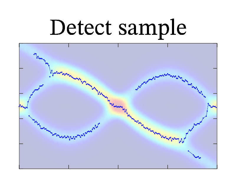
Next: diffract sample, Previous: detect sample, Up: All samples [Contents][Index]
Function dew is similar to vect but use drops instead of arrows.
MGL code:
call 'prepare2v' subplot 1 1 0 '':title 'Dew plot':light on:box:dew a b
C++ code:
void smgl_dew(mglGraph *gr)
{
mglData a,b; mgls_prepare2v(&a,&b);
if(big!=3) {gr->SubPlot(1,1,0,""); gr->Title("Dew plot");}
gr->Box(); gr->Light(true); gr->Dew(a,b);
}
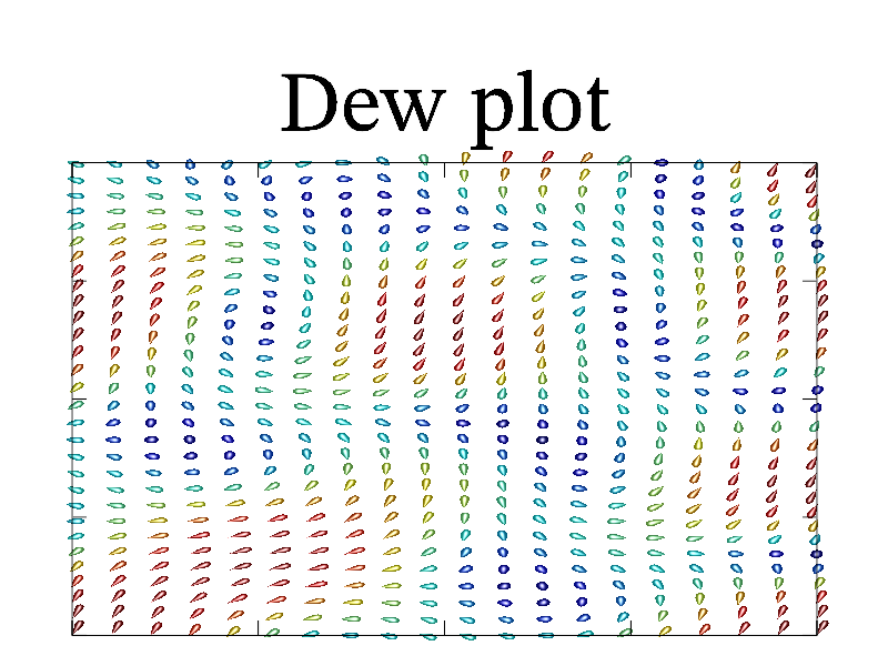
Next: dilate sample, Previous: dew sample, Up: All samples [Contents][Index]
MGL code:
define n 32 #number of points define m 20 # number of iterations define dt 0.01 # time step new res n m+1 ranges -1 1 0 m*dt 0 1 #tridmat periodic variant new !a n 'i',dt*(n/2)^2/2 copy !b !(1-2*a) new !u n 'exp(-6*x^2)' put res u all 0 for $i 0 m tridmat u a b a u 'xdc' put res u all $i+1 next subplot 2 2 0 '<_':title 'Tridmat, periodic b.c.' axis:box:dens res #fourier variant new k n:fillsample k 'xk' copy !e !exp(-i1*dt*k^2) new !u n 'exp(-6*x^2)' put res u all 0 for $i 0 m fourier u 'x' multo u e fourier u 'ix' put res u all $i+1 next subplot 2 2 1 '<_':title 'Fourier method' axis:box:dens res #tridmat zero variant new !u n 'exp(-6*x^2)' put res u all 0 for $i 0 m tridmat u a b a u 'xd' put res u all $i+1 next subplot 2 2 2 '<_':title 'Tridmat, zero b.c.' axis:box:dens res #diffract exp variant new !u n 'exp(-6*x^2)' define q dt*(n/2)^2/8 # need q<0.4 !!! put res u all 0 for $i 0 m for $j 1 8 # due to smaller dt diffract u 'xe' q next put res u all $i+1 next subplot 2 2 3 '<_':title 'Diffract, exp b.c.' axis:box:dens res
C++ code:
void smgl_diffract(mglGraph *gr)
{
long n=32; // number of points
long m=20; // number of iterations
double dt=0.01; // time step
mglData res(n,m+1);
gr->SetRanges(-1,1, 0,m*dt, 0,1);
// tridmat periodic variant
mglDataC a(n), b(n); a = dual(0,dt*n*n/8);
for(long i=0;i<n;i++) b.a[i] = mreal(1)-mreal(2)*a.a[i];
mglDataC u(n); gr->Fill(u,"exp(-6*x^2)"); res.Put(u,-1,0);
for(long i=0;i<m;i++)
{
u = mglTridMatC(a,b,a,u,"xdc");
res.Put(u,-1,i+1);
}
gr->SubPlot(2,2,0,"<_"); gr->Title("Tridmat, periodic b.c.");
gr->Axis(); gr->Box(); gr->Dens(res);
// fourier variant
mglData k(n); k.FillSample("xk");
mglDataC e(n); for(long i=0;i<n;i++) e.a[i] = exp(-dual(0,dt*k.a[i]*k.a[i]));
gr->Fill(u,"exp(-6*x^2)"); res.Put(u,-1,0);
for(long i=0;i<m;i++)
{
u.FFT("x"); u *= e; u.FFT("ix");
res.Put(u,-1,i+1);
}
gr->SubPlot(2,2,1,"<_"); gr->Title("Fourier method");
gr->Axis(); gr->Box(); gr->Dens(res);
// tridmat zero variant
gr->Fill(u,"exp(-6*x^2)"); res.Put(u,-1,0);
for(long i=0;i<m;i++)
{
u = mglTridMatC(a,b,a,u,"xd");
res.Put(u,-1,i+1);
}
gr->SubPlot(2,2,2,"<_"); gr->Title("Tridmat, zero b.c.");
gr->Axis(); gr->Box(); gr->Dens(res);
// diffract exp variant
gr->Fill(u,"exp(-6*x^2)"); res.Put(u,-1,0);
double q=dt*n*n/4/8; // NOTE: need q<0.4 !!!
for(long i=0;i<m;i++)
{
for(long j=0;j<8;j++) // due to smaller dt
u.Diffraction("xe",q);
res.Put(u,-1,i+1);
}
gr->SubPlot(2,2,3,"<_"); gr->Title("Diffract, exp b.c.");
gr->Axis(); gr->Box(); gr->Dens(res);
}

Next: dots sample, Previous: diffract sample, Up: All samples [Contents][Index]
MGL code:
subplot 2 2 0:title 'Dilate&Erode 1D sample' new y 11:put y 1 5 ranges 0 10 0 1:axis:box plot y 'b*' dilate y 0.5 2 plot y 'rs' erode y 0.5 1 plot y 'g#o' subplot 2 2 1:title 'Dilate&Erode 2D sample':rotate 40 60 ranges 0 10 0 10 0 3 axis:box new z 11 11:put z 3 5 5 boxs z 'b':boxs z 'k#' dilate z 1 2 boxs z 'r':boxs z 'k#' erode z 1 1 boxs 2*z 'g':boxs 2*z 'k#' subplot 2 2 2 text 0.5 0.7 'initial' 'ba';size -2 text 0.5 0.5 'dilate=2' 'ra';size -2 text 0.5 0.3 'erode=1' 'ga';size -2 subplot 2 2 3:title 'Dilate&Erode 3D sample' rotate 60 50:light on:alpha on ranges 0 10 0 10 0 10:crange 0 3 axis:box new a 11 11 11:put a 3 5 5 5 surf3a a a 1.5 'b' dilate a 1 2 surf3a a a 0.5 'r' erode a 1 1 surf3a 2*a 2*a 1 'g'
C++ code:
void smgl_dilate(mglGraph *gr)
{
mglData y(11), z(11,11), a(11,11,11);
y.a[5]=1; z.a[5+11*5]=a.a[5+11*(5+11*5)] = 3;
if(big!=3) { gr->SubPlot(2,2,0); gr->Title("Dilate&Erode 1D sample"); }
else gr->SubPlot(1,1,0,"");
gr->SetRanges(0,10,0,1); gr->Axis(); gr->Box(); gr->Plot(y,"b*");
y.Dilate(1,2); gr->Plot(y,"rs");
y.Erode(1,1); gr->Plot(y,"g#o");
if(big==3) return;
gr->SubPlot(2,2,1); gr->Title("Dilate&Erode 2D sample");
gr->Rotate(40,60); gr->SetRanges(0,10,0,10,0,3);
gr->Axis(); gr->Box(); gr->Boxs(z,"b"); gr->Boxs(z,"k#");
z.Dilate(1,2); gr->Boxs(z,"r"); gr->Boxs(z,"k#");
z.Erode(1,1); z*=2; gr->Boxs(z,"g"); gr->Boxs(z,"k#");
gr->SubPlot(2,2,2);
gr->Puts(0.5,0.7,"initial","ba",-2);
gr->Puts(0.5,0.5,"dilate=2","ra",-2);
gr->Puts(0.5,0.3,"erode=1","ga",-2);
gr->SubPlot(2,2,3); gr->Title("Dilate&Erode 3D sample");
gr->Rotate(60,50); gr->Alpha(true); gr->Light(true);
gr->SetRanges(0,10,0,10,0,10); gr->SetRange('c',0,3);
gr->Axis(); gr->Box(); gr->Surf3A(1.5,a,a,"b");
a.Dilate(1,2); gr->Surf3A(0.5,a,a,"r");
a.Erode(1,1); a*=2; gr->Surf3A(1,a,a,"g");
}
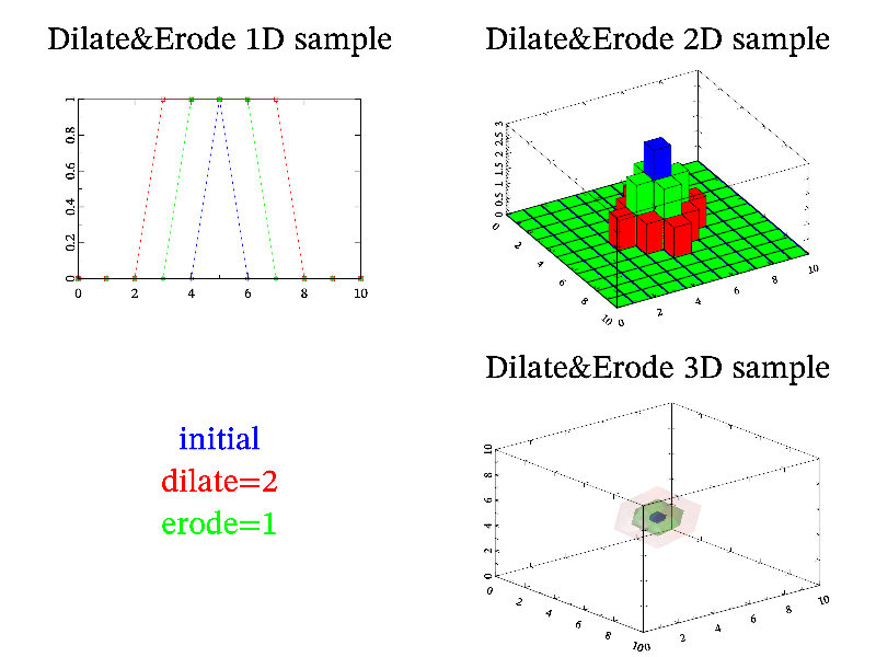
Next: earth sample, Previous: dilate sample, Up: All samples [Contents][Index]
Function dots is another way to draw irregular points. Dots use color scheme for coloring (see Color scheme).
MGL code:
new t 2000 'pi*(rnd-0.5)':new f 2000 '2*pi*rnd' copy x 0.9*cos(t)*cos(f):copy y 0.9*cos(t)*sin(f):copy z 0.6*sin(t):copy c cos(2*t) subplot 2 2 0:title 'Dots sample':rotate 50 60 box:dots x y z alpha on subplot 2 2 1:title 'add transparency':rotate 50 60 box:dots x y z c subplot 2 2 2:title 'add colorings':rotate 50 60 box:dots x y z x c subplot 2 2 3:title 'Only coloring':rotate 50 60 box:tens x y z x ' .'
C++ code:
void smgl_dots(mglGraph *gr)
{
int i, n=1000;
mglData x(n),y(n),z(n),c(n);
for(i=0;i<n;i++)
{
double t=M_PI*(mgl_rnd()-0.5), f=2*M_PI*mgl_rnd();
x.a[i] = 0.9*cos(t)*cos(f);
y.a[i] = 0.9*cos(t)*sin(f);
z.a[i] = 0.6*sin(t);
c.a[i] = cos(2*t);
}
if(big!=3) { gr->SubPlot(2,2,0); gr->Title("Dots sample"); }
gr->Rotate(50,60); gr->Box(); gr->Dots(x,y,z);
if(big==3) return;
gr->Alpha(true);
gr->SubPlot(2,2,1); gr->Title("add transparency"); gr->Rotate(50,60); gr->Box(); gr->Dots(x,y,z,c);
gr->SubPlot(2,2,2); gr->Title("add coloring"); gr->Rotate(50,60); gr->Box(); gr->Dots(x,y,z,x,c);
gr->SubPlot(2,2,3); gr->Title("Only coloring"); gr->Rotate(50,60); gr->Box(); gr->Tens(x,y,z,x," .");
}

Next: error sample, Previous: dots sample, Up: All samples [Contents][Index]
Example of Earth map by using import.
MGL code:
import dat 'Equirectangular-projection.jpg' 'BbGYw' -1 1 subplot 1 1 0 '<>':title 'Earth in 3D':rotate 40 60 copy phi dat 'pi*x':copy tet dat 'pi*y/2' copy x cos(tet)*cos(phi) copy y cos(tet)*sin(phi) copy z sin(tet) light on surfc x y z dat 'BbGYw' contp [-0.51,-0.51] x y z dat 'y'
C++ code:
void smgl_earth(mglGraph *gr)
{
mglData dat; dat.Import("Equirectangular-projection.jpg","BbGYw",-1,1);
// Calc proper 3d coordinates from projection
mglData phi(dat.nx,dat.ny); phi.Fill(-M_PI,M_PI);
mglData tet(dat.nx,dat.ny); tet.Fill(-M_PI/2,M_PI/2,'y');
mglData x(dat.nx,dat.ny), y(dat.nx,dat.ny), z(dat.nx,dat.ny);
#pragma omp parallel for
for(long i=0;i<dat.nx*dat.ny;i++)
{ x.a[i] = cos(tet.a[i])*cos(phi.a[i]);
y.a[i] = cos(tet.a[i])*sin(phi.a[i]);
z.a[i] = sin(tet.a[i]); }
gr->SubPlot(1,1,0,"<>");
if(big!=3) gr->Title("Earth in 3D");
gr->Rotate(40,60); gr->Light(true);
gr->SurfC(x,y,z,dat,"BbGYw");
mglData vals(1); vals.a[0]=-0.51;
gr->ContP(vals, x,y,z,dat,"y");
}

Next: error2 sample, Previous: earth sample, Up: All samples [Contents][Index]
Function error draw error boxes around the points. You can draw default boxes or semi-transparent symbol (like marker, see Line styles). Also you can set individual color for each box. See also error2 sample.
MGL code:
call 'prepare1d' new y 50 '0.7*sin(pi*x-pi) + 0.5*cos(3*pi*(x+1)/2) + 0.2*sin(pi*(x+1)/2)' new x0 10 'x + 0.1*rnd-0.05':new ex 10 '0.1':new ey 10 '0.2' new y0 10 '0.7*sin(pi*x-pi) + 0.5*cos(3*pi*(x+1)/2) + 0.2*sin(pi*(x+1)/2) + 0.2*rnd-0.1' subplot 2 2 0 '':title 'Error plot (default)':box:plot y:error x0 y0 ex ey 'k' subplot 2 2 1 '':title '"!" style; no e_x':box:plot y:error x0 y0 ey 'o!rgb' subplot 2 2 2 '':title '"\@" style':alpha on:box:plot y:error x0 y0 ex ey '@'; alpha 0.5 subplot 2 2 3:title '3d variant':rotate 50 60:axis for $1 0 9 errbox 2*rnd-1 2*rnd-1 2*rnd-1 0.2 0.2 0.2 'bo' next
C++ code:
void smgl_error2(mglGraph *gr)
{
mglData x0(10), y0(10), ex(10), ey(10);
for(int i=0;i<10;i++)
{ x0.a[i] = mgl_rnd(); y0.a[i] = mgl_rnd(); ey.a[i] = ex.a[i] = 0.1; }
gr->SetRanges(0,1,0,1); gr->Alpha(true);
gr->SubPlot(4,3,0,""); gr->Box(); gr->Error(x0,y0,ex,ey,"#+@");
gr->SubPlot(4,3,1,""); gr->Box(); gr->Error(x0,y0,ex,ey,"#x@");
gr->SubPlot(4,3,2,""); gr->Box(); gr->Error(x0,y0,ex,ey,"#s@","alpha 0.5");
gr->SubPlot(4,3,3,""); gr->Box(); gr->Error(x0,y0,ex,ey,"s@");
gr->SubPlot(4,3,4,""); gr->Box(); gr->Error(x0,y0,ex,ey,"d@");
gr->SubPlot(4,3,5,""); gr->Box(); gr->Error(x0,y0,ex,ey,"#d@","alpha 0.5");
gr->SubPlot(4,3,6,""); gr->Box(); gr->Error(x0,y0,ex,ey,"+@");
gr->SubPlot(4,3,7,""); gr->Box(); gr->Error(x0,y0,ex,ey,"x@");
gr->SubPlot(4,3,8,""); gr->Box(); gr->Error(x0,y0,ex,ey,"o@");
gr->SubPlot(4,3,9,""); gr->Box(); gr->Error(x0,y0,ex,ey,"#o@","alpha 0.5");
gr->SubPlot(4,3,10,""); gr->Box(); gr->Error(x0,y0,ex,ey,"#.@");
gr->SubPlot(4,3,11,""); gr->Box(); gr->Error(x0,y0,ex,ey);
}
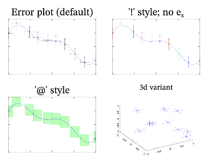
Next: export sample, Previous: error sample, Up: All samples [Contents][Index]
Example of error kinds.
MGL code:
new x0 10 'rnd':new ex 10 '0.1' new y0 10 'rnd':new ey 10 '0.1' ranges 0 1 0 1 subplot 4 3 0 '':box:error x0 y0 ex ey '#+@' subplot 4 3 1 '':box:error x0 y0 ex ey '#x@' subplot 4 3 2 '':box:error x0 y0 ex ey '#s@'; alpha 0.5 subplot 4 3 3 '':box:error x0 y0 ex ey 's@' subplot 4 3 4 '':box:error x0 y0 ex ey 'd@' subplot 4 3 5 '':box:error x0 y0 ex ey '#d@'; alpha 0.5 subplot 4 3 6 '':box:error x0 y0 ex ey '+@' subplot 4 3 7 '':box:error x0 y0 ex ey 'x@' subplot 4 3 8 '':box:error x0 y0 ex ey 'o@' subplot 4 3 9 '':box:error x0 y0 ex ey '#o@'; alpha 0.5 subplot 4 3 10 '':box:error x0 y0 ex ey '#.@' subplot 4 3 11 '':box:error x0 y0 ex ey; alpha 0.5
C++ code:
void smgl_error2(mglGraph *gr)
{
mglData x0(10), y0(10), ex(10), ey(10);
for(int i=0;i<10;i++)
{ x0.a[i] = mgl_rnd(); y0.a[i] = mgl_rnd(); ey.a[i] = ex.a[i] = 0.1; }
gr->SetRanges(0,1,0,1); gr->Alpha(true);
gr->SubPlot(4,3,0,""); gr->Box(); gr->Error(x0,y0,ex,ey,"#+@");
gr->SubPlot(4,3,1,""); gr->Box(); gr->Error(x0,y0,ex,ey,"#x@");
gr->SubPlot(4,3,2,""); gr->Box(); gr->Error(x0,y0,ex,ey,"#s@","alpha 0.5");
gr->SubPlot(4,3,3,""); gr->Box(); gr->Error(x0,y0,ex,ey,"s@");
gr->SubPlot(4,3,4,""); gr->Box(); gr->Error(x0,y0,ex,ey,"d@");
gr->SubPlot(4,3,5,""); gr->Box(); gr->Error(x0,y0,ex,ey,"#d@","alpha 0.5");
gr->SubPlot(4,3,6,""); gr->Box(); gr->Error(x0,y0,ex,ey,"+@");
gr->SubPlot(4,3,7,""); gr->Box(); gr->Error(x0,y0,ex,ey,"x@");
gr->SubPlot(4,3,8,""); gr->Box(); gr->Error(x0,y0,ex,ey,"o@");
gr->SubPlot(4,3,9,""); gr->Box(); gr->Error(x0,y0,ex,ey,"#o@","alpha 0.5");
gr->SubPlot(4,3,10,""); gr->Box(); gr->Error(x0,y0,ex,ey,"#.@");
gr->SubPlot(4,3,11,""); gr->Box(); gr->Error(x0,y0,ex,ey);
}
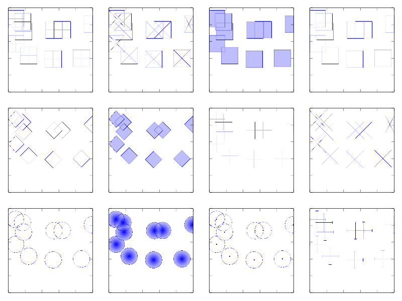
Next: fall sample, Previous: error2 sample, Up: All samples [Contents][Index]
Example of data export and import.
MGL code:
new a 100 100 'x^2*y':new b 100 100 export a 'test_data.png' 'BbcyrR' -1 1 import b 'test_data.png' 'BbcyrR' -1 1 subplot 2 1 0 '':title 'initial':box:dens a subplot 2 1 1 '':title 'imported':box:dens b
C++ code:
void smgl_export(mglGraph *gr) // basic data operations
{
mglData a(100,100), b; gr->Fill(a,"x^2*y");
a.Export("test_data.png","BbcyrR");
b.Import("test_data.png","BbcyrR",-1,1);
gr->SubPlot(2,1,0,""); gr->Title("initial"); gr->Box(); gr->Dens(a);
gr->SubPlot(2,1,1,""); gr->Title("imported"); gr->Box(); gr->Dens(b);
}
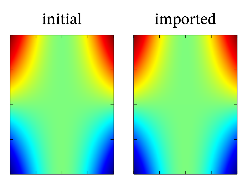
Next: fexport sample, Previous: export sample, Up: All samples [Contents][Index]
Function fall draw waterfall surface. You can use meshnum for changing number of lines to be drawn. Also you can use ‘x’ style for drawing lines in other direction.
MGL code:
call 'prepare2d' title 'Fall plot':rotate 50 60:box:fall a
C++ code:
void smgl_fall(mglGraph *gr)
{
mglData a; mgls_prepare2d(&a);
if(big!=3) gr->Title("Fall plot");
gr->Rotate(50,60); gr->Box(); gr->Fall(a);
}

Next: fit sample, Previous: fall sample, Up: All samples [Contents][Index]
Example of write to different file formats.
MGL code:
subplot 3 2 0:define y 0.95
define d 0.3:define x0 0.2:define x1 0.5:define x2 0.6
line x0 1-0*d x1 1-0*d 'k-':text x2 y-0*d 'Solid `-`' ':rL'
line x0 1-1*d x1 1-1*d 'k|':text x2 y-1*d 'Long Dash `|`' ':rL'
line x0 1-2*d x1 1-2*d 'k;':text x2 y-2*d 'Dash 1;`' ':rL'
line x0 1-3*d x1 1-3*d 'k=':text x2 y-3*d 'Small dash `=`' ':rL'
line x0 1-4*d x1 1-4*d 'kj':text x2 y-4*d 'Dash-dot `j`' ':rL'
line x0 1-5*d x1 1-5*d 'ki':text x2 y-5*d 'Small dash-dot `i`' ':rL'
line x0 1-6*d x1 1-6*d 'k:':text x2 y-6*d 'Dots `:`' ':rL'
line x0 1-7*d x1 1-7*d 'k ':text x2 y-7*d 'None ``' ':rL'
define d 0.25:define x0 -0.8:define x1 -1:define x2 -0.05
ball x1 5*d 'k.':text x0 5*d '.' ':rL'
ball x1 4*d 'k+':text x0 4*d '+' ':rL'
ball x1 3*d 'kx':text x0 3*d 'x' ':rL'
ball x1 2*d 'k*':text x0 2*d '*' ':rL'
ball x1 d 'ks':text x0 d 's' ':rL'
ball x1 0 'kd':text x0 0 'd' ':rL'
ball x1 -d 0 'ko':text x0 y-d 'o' ':rL'
ball x1 -2*d 0 'k^':text x0 -2*d '\^' ':rL'
ball x1 -3*d 0 'kv':text x0 -3*d 'v' ':rL'
ball x1 -4*d 0 'k<':text x0 -4*d '<' ':rL'
ball x1 -5*d 0 'k>':text x0 -5*d '>' ':rL'
define x0 -0.3:define x1 -0.5
ball x1 5*d 'k#.':text x0 5*d '\#.' ':rL'
ball x1 4*d 'k#+':text x0 4*d '\#+' ':rL'
ball x1 3*d 'k#x':text x0 3*d '\#x' ':rL'
ball x1 2*d 'k#*':text x0 2*d '\#*' ':rL'
ball x1 d 'k#s':text x0 d '\#s' ':rL'
ball x1 0 'k#d':text x0 0 '\#d' ':rL'
ball x1 -d 0 'k#o':text x0 -d '\#o' ':rL'
ball x1 -2*d 0 'k#^':text x0 -2*d '\#\^' ':rL'
ball x1 -3*d 0 'k#v':text x0 -3*d '\#v' ':rL'
ball x1 -4*d 0 'k#<':text x0 -4*d '\#<' ':rL'
ball x1 -5*d 0 'k#>':text x0 -5*d '\#>' ':rL'
subplot 3 2 1
define a 0.1:define b 0.4:define c 0.5
line a 1 b 1 'k-A':text c 1 'Style `A` or `A\_`' ':rL'
line a 0.8 b 0.8 'k-V':text c 0.8 'Style `V` or `V\_`' ':rL'
line a 0.6 b 0.6 'k-K':text c 0.6 'Style `K` or `K\_`' ':rL'
line a 0.4 b 0.4 'k-I':text c 0.4 'Style `I` or `I\_`' ':rL'
line a 0.2 b 0.2 'k-D':text c 0.2 'Style `D` or `D\_`' ':rL'
line a 0 b 0 'k-S':text c 0 'Style `S` or `S\_`' ':rL'
line a -0.2 b -0.2 'k-O':text c -0.2 'Style `O` or `O\_`' ':rL'
line a -0.4 b -0.4 'k-T':text c -0.4 'Style `T` or `T\_`' ':rL'
line a -0.6 b -0.6 'k-_':text c -0.6 'Style `\_` or none' ':rL'
line a -0.8 b -0.8 'k-AS':text c -0.8 'Style `AS`' ':rL'
line a -1 b -1 'k-_A':text c -1 'Style `\_A`' ':rL'
define a -1:define b -0.7:define c -0.6
line a 1 b 1 'kAA':text c 1 'Style `AA`' ':rL'
line a 0.8 b 0.8 'kVV':text c 0.8 'Style `VV`' ':rL'
line a 0.6 b 0.6 'kKK':text c 0.6 'Style `KK`' ':rL'
line a 0.4 b 0.4 'kII':text c 0.4 'Style `II`' ':rL'
line a 0.2 b 0.2 'kDD':text c 0.2 'Style `DD`' ':rL'
line a 0 b 0 'kSS':text c 0 'Style `SS`' ':rL'
line a -0.2 b -0.2 'kOO':text c -0.2 'Style `OO`' ':rL'
line a -0.4 b -0.4 'kTT':text c -0.4 'Style `TT`' ':rL'
line a -0.6 b -0.6 'k-__':text c -0.6 'Style `\_\_`' ':rL'
line a -0.8 b -0.8 'k-VA':text c -0.8 'Style `VA`' ':rL'
line a -1 b -1 'k-AV':text c -1 'Style `AV`' ':rL'
subplot 3 2 2
#LENUQ
facez -1 -1 0 0.4 0.3 'L#':text -0.8 -0.9 'L' 'w:C' -1.4
facez -0.6 -1 0 0.4 0.3 'E#':text -0.4 -0.9 'E' 'w:C' -1.4
facez -0.2 -1 0 0.4 0.3 'N#':text 0 -0.9 'N' 'w:C' -1.4
facez 0.2 -1 0 0.4 0.3 'U#':text 0.4 -0.9 'U' 'w:C' -1.4
facez 0.6 -1 0 0.4 0.3 'Q#':text 0.8 -0.9 'Q' 'w:C' -1.4
#lenuq
facez -1 -0.7 0 0.4 0.3 'l#':text -0.8 -0.6 'l' 'k:C' -1.4
facez -0.6 -0.7 0 0.4 0.3 'e#':text -0.4 -0.6 'e' 'k:C' -1.4
facez -0.2 -0.7 0 0.4 0.3 'n#':text 0 -0.6 'n' 'k:C' -1.4
facez 0.2 -0.7 0 0.4 0.3 'u#':text 0.4 -0.6 'u' 'k:C' -1.4
facez 0.6 -0.7 0 0.4 0.3 'q#':text 0.8 -0.6 'q' 'k:C' -1.4
#CMYkP
facez -1 -0.4 0 0.4 0.3 'C#':text -0.8 -0.3 'C' 'w:C' -1.4
facez -0.6 -0.4 0 0.4 0.3 'M#':text -0.4 -0.3 'M' 'w:C' -1.4
facez -0.2 -0.4 0 0.4 0.3 'Y#':text 0 -0.3 'Y' 'w:C' -1.4
facez 0.2 -0.4 0 0.4 0.3 'k#':text 0.4 -0.3 'k' 'w:C' -1.4
facez 0.6 -0.4 0 0.4 0.3 'P#':text 0.8 -0.3 'P' 'w:C' -1.4
#cmywp
facez -1 -0.1 0 0.4 0.3 'c#':text -0.8 0 'c' 'k:C' -1.4
facez -0.6 -0.1 0 0.4 0.3 'm#':text -0.4 0 'm' 'k:C' -1.4
facez -0.2 -0.1 0 0.4 0.3 'y#':text 0 0 'y' 'k:C' -1.4
facez 0.2 -0.1 0 0.4 0.3 'w#':text 0.4 0 'w' 'k:C' -1.4
facez 0.6 -0.1 0 0.4 0.3 'p#':text 0.8 0 'p' 'k:C' -1.4
#BGRHW
facez -1 0.2 0 0.4 0.3 'B#':text -0.8 0.3 'B' 'w:C' -1.4
facez -0.6 0.2 0 0.4 0.3 'G#':text -0.4 0.3 'G' 'w:C' -1.4
facez -0.2 0.2 0 0.4 0.3 'R#':text 0 0.3 'R' 'w:C' -1.4
facez 0.2 0.2 0 0.4 0.3 'H#':text 0.4 0.3 'H' 'w:C' -1.4
facez 0.6 0.2 0 0.4 0.3 'W#':text 0.8 0.3 'W' 'w:C' -1.4
#bgrhw
facez -1 0.5 0 0.4 0.3 'b#':text -0.8 0.6 'b' 'k:C' -1.4
facez -0.6 0.5 0 0.4 0.3 'g#':text -0.4 0.6 'g' 'k:C' -1.4
facez -0.2 0.5 0 0.4 0.3 'r#':text 0 0.6 'r' 'k:C' -1.4
facez 0.2 0.5 0 0.4 0.3 'h#':text 0.4 0.6 'h' 'k:C' -1.4
facez 0.6 0.5 0 0.4 0.3 'w#':text 0.8 0.6 'w' 'k:C' -1.4
#brighted
facez -1 0.8 0 0.4 0.3 '{r1}#':text -0.8 0.9 '\{r1\}' 'w:C' -1.4
facez -0.6 0.8 0 0.4 0.3 '{r3}#':text -0.4 0.9 '\{r3\}' 'w:C' -1.4
facez -0.2 0.8 0 0.4 0.3 '{r5}#':text 0 0.9 '\{r5\}' 'k:C' -1.4
facez 0.2 0.8 0 0.4 0.3 '{r7}#':text 0.4 0.9 '\{r7\}' 'k:C' -1.4
facez 0.6 0.8 0 0.4 0.3 '{r9}#':text 0.8 0.9 '\{r9\}' 'k:C' -1.4
# HEX
facez -1 -1.3 0 1 0.3 '{xff9966}#':text -0.5 -1.2 '\{xff9966\}' 'k:C' -1.4
facez 0 -1.3 0 1 0.3 '{x83CAFF}#':text 0.5 -1.2 '\{x83caff\}' 'k:C' -1.4
subplot 3 2 3
for $i 0 9
line -1 0.2*$i-1 1 0.2*$i-1 'r','0'+$i
text 1.05 0.2*$i-1 '0'+$i ':L'
next
subplot 3 2 4:title 'TriPlot sample':rotate 50 60
list tt 0 1 2 | 0 1 3 | 0 2 3 | 1 2 3
list xt -1 1 0 0:list yt -1 -1 1 0:list zt -1 -1 -1 1:light on
triplot tt xt yt zt 'b':triplot tt xt yt zt 'k#'
subplot 3 2 5:new r 4 'i+1':ranges 1 4 1 4
axis:mark r r 's':plot r 'b'
write 'fexport.jpg':#write 'fexport.png'
write 'fexport.bmp':write 'fexport.tga'
write 'fexport.eps':write 'fexport.svg'
write 'fexport.gif':write 'fexport.xyz'
write 'fexport.stl':write 'fexport.off'
write 'fexport.tex':write 'fexport.obj'
write 'fexport.prc':write 'fexport.json'
write 'fexport.mgld'
C++ code:
void smgl_fexport(mglGraph *gr) // test file export
{
all_prims(gr);
gr->WriteJPEG("fexport.jpg");
// gr->WritePNG("fexport.png");
gr->WriteBMP("fexport.bmp");
gr->WriteTGA("fexport.tga");
gr->WriteEPS("fexport.eps");
gr->WriteSVG("fexport.svg");
gr->WriteGIF("fexport.gif");
gr->WriteXYZ("fexport.xyz");
gr->WriteSTL("fexport.stl");
gr->WriteOFF("fexport.off");
gr->WriteTEX("fexport.tex");
gr->WriteOBJ("fexport.obj");
gr->WritePRC("fexport.prc");
gr->WriteJSON("fexport.json");
gr->ExportMGLD("fexport.mgld");
gr->Clf();
gr->ImportMGLD("fexport.mgld");
}

Next: flame2d sample, Previous: fexport sample, Up: All samples [Contents][Index]
Example of nonlinear fit.
MGL code:
new dat 100 '0.4*rnd+0.1+sin(2*pi*x)' new in 100 '0.3+sin(2*pi*x)' list ini 1 1 3:fit res dat 'a+b*sin(c*x)' 'abc' ini title 'Fitting sample':yrange -2 2:box:axis:plot dat 'k. ' plot res 'r':plot in 'b' text -0.9 -1.3 'fitted:' 'r:L' putsfit 0 -1.8 'y = ' 'r':text 0 2.2 'initial: y = 0.3+sin(2\pi x)' 'b'
C++ code:
void smgl_fit(mglGraph *gr) // nonlinear fitting
{
mglData dat(100), in(100), res;
gr->Fill(dat,"0.4*rnd+0.1+sin(2*pi*x)");
gr->Fill(in,"0.3+sin(2*pi*x)");
double ini[3] = {1,1,3};
mglData Ini(3,ini);
res = gr->Fit(dat, "a+b*sin(c*x)", "abc", Ini);
if(big!=3) gr->Title("Fitting sample");
gr->SetRange('y',-2,2); gr->Box(); gr->Plot(dat, "k. ");
gr->Axis(); gr->Plot(res, "r"); gr->Plot(in, "b");
gr->Puts(mglPoint(-0.9, -1.3), "fitted:", "r:L");
gr->PutsFit(mglPoint(0, -1.8), "y = ", "r");
gr->Puts(mglPoint(0, 2.2), "initial: y = 0.3+sin(2\\pi x)", "b");
// gr->SetRanges(mglPoint(-1,-1,-1),mglPoint(1,1,1)); gr->SetOrigin(0,0,0);
}
Next: flow sample, Previous: fit sample, Up: All samples [Contents][Index]
Function flame2d generate points for flame fractals in 2d case.
MGL code:
list A [0.33,0,0,0.33,0,0,0.2] [0.33,0,0,0.33,0.67,0,0.2] [0.33,0,0,0.33,0.33,0.33,0.2]\ [0.33,0,0,0.33,0,0.67,0.2] [0.33,0,0,0.33,0.67,0.67,0.2] new B 2 3 A.ny '0.3' put B 3 0 0 -1 put B 3 0 1 -1 put B 3 0 2 -1 flame2d fx fy A B 1000000 subplot 1 1 0 '<_':title 'Flame2d sample' ranges fx fy:box:axis plot fx fy 'r#o ';size 0.05
C++ code:
void smgl_flame2d(mglGraph *gr)
{
mglData A, B(2,3,5);
A.SetList(35, 0.33,0.,0.,0.33,0.,0.,0.2, 0.33,0.,0.,0.33,0.67,0.,0.2, 0.33,0.,0.,0.33,0.33,0.33,0.2,
0.33,0.,0.,0.33,0.,0.67,0.2, 0.33,0.,0.,0.33,0.67,0.67,0.2);
A.Rearrange(7);
for(long i=0;i<2*3*5;i++) B.a[i] = 0.3;
for(long i=0;i<5;i++) B.a[2*3*i] = B.a[2*3*i+1*2] = B.a[2*3*i+2*2] = 3;
mglData f(mglFlame2d(A,B,1000000));
gr->SubPlot(1,1,0,"<_");
if(big!=3) gr->Title("Flame2d sample");
gr->SetRanges(f.SubData(0), f.SubData(1));
gr->Axis(); gr->Box();
gr->Plot(f.SubData(0), f.SubData(1),"r#o ","size 0.05");
}
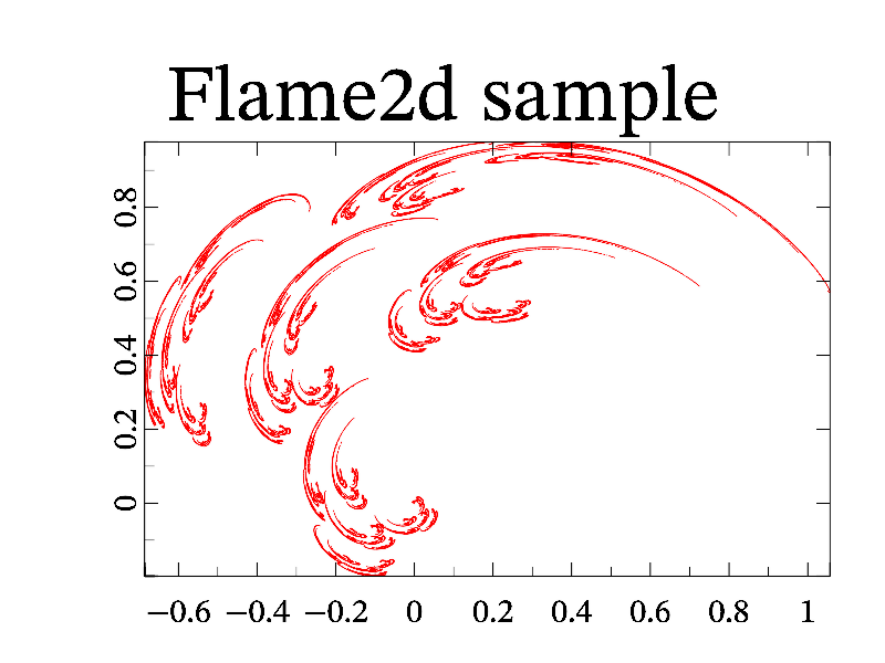
Next: flow3 sample, Previous: flame2d sample, Up: All samples [Contents][Index]
Function flow is another standard way to visualize vector fields – it draw lines (threads) which is tangent to local vector field direction. MathGL draw threads from edges of bounding box and from central slices. Sometimes it is not most appropriate variant – you may want to use flowp to specify manual position of threads. The color scheme is used for coloring (see Color scheme). At this warm color corresponds to normal flow (like attractor), cold one corresponds to inverse flow (like source).
MGL code:
call 'prepare2v' call 'prepare3v' subplot 2 2 0 '':title 'Flow plot (default)':box:flow a b subplot 2 2 1 '':title '"v" style':box:flow a b 'v' subplot 2 2 2 '':title '"#" and "." styles':box:flow a b '#':flow a b '.2k' subplot 2 2 3:title '3d variant':rotate 50 60:box:flow ex ey ez
C++ code:
void smgl_flow(mglGraph *gr)
{
mglData a,b; mgls_prepare2v(&a,&b);
if(big!=3) {gr->SubPlot(2,2,0,""); gr->Title("Flow plot (default)");}
gr->Box(); gr->Flow(a,b);
if(big==3) return;
gr->SubPlot(2,2,1,""); gr->Title("'v' style");
gr->Box(); gr->Flow(a,b,"v");
gr->SubPlot(2,2,2,""); gr->Title("'\\#' and '.' styles");
gr->Box(); gr->Flow(a,b,"#"); gr->Flow(a,b,".2k");
mglData ex,ey,ez; mgls_prepare3v(&ex,&ey,&ez);
gr->SubPlot(2,2,3); gr->Title("3d variant"); gr->Rotate(50,60);
gr->Box(); gr->Flow(ex,ey,ez);
}
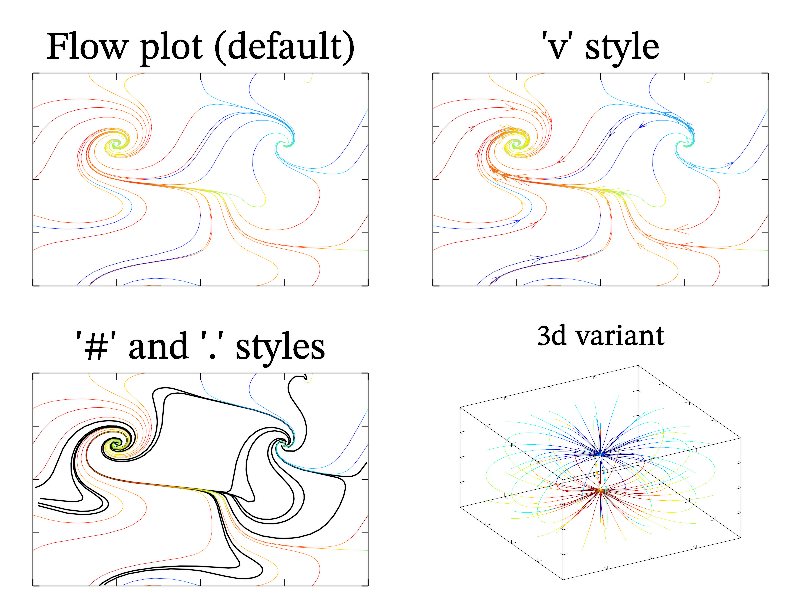
Next: fog sample, Previous: flow sample, Up: All samples [Contents][Index]
Function flow3 draw flow threads, which start from given plane.
MGL code:
call 'prepare3v' subplot 2 2 0:title 'Flow3 plot (default)':rotate 50 60:box flow3 ex ey ez subplot 2 2 1:title '"v" style, from boundary':rotate 50 60:box flow3 ex ey ez 'v' 0 subplot 2 2 2:title '"t" style':rotate 50 60:box flow3 ex ey ez 't' 0 subplot 2 2 3:title 'from \i z planes':rotate 50 60:box flow3 ex ey ez 'z' 0 flow3 ex ey ez 'z' 9
C++ code:
void smgl_flow3(mglGraph *gr)
{
mglData ex,ey,ez; mgls_prepare3v(&ex,&ey,&ez);
if(big!=3) {gr->SubPlot(2,2,0); gr->Title("Flow3 plot (default)");}
gr->Rotate(50,60); gr->Box(); gr->Flow3(ex,ey,ez);
if(big==3) return;
gr->SubPlot(2,2,1); gr->Title("'v' style, from boundary");
gr->Rotate(50,60); gr->Box(); gr->Flow3(ex,ey,ez,"v",0);
gr->SubPlot(2,2,2); gr->Title("'t' style");
gr->Rotate(50,60); gr->Box(); gr->Flow3(ex,ey,ez,"t",0);
gr->SubPlot(2,2,3); gr->Title("from \\i z planes");
gr->Rotate(50,60); gr->Box(); gr->Flow3(ex,ey,ez,"z",0); gr->Flow3(ex,ey,ez,"z",9);
}
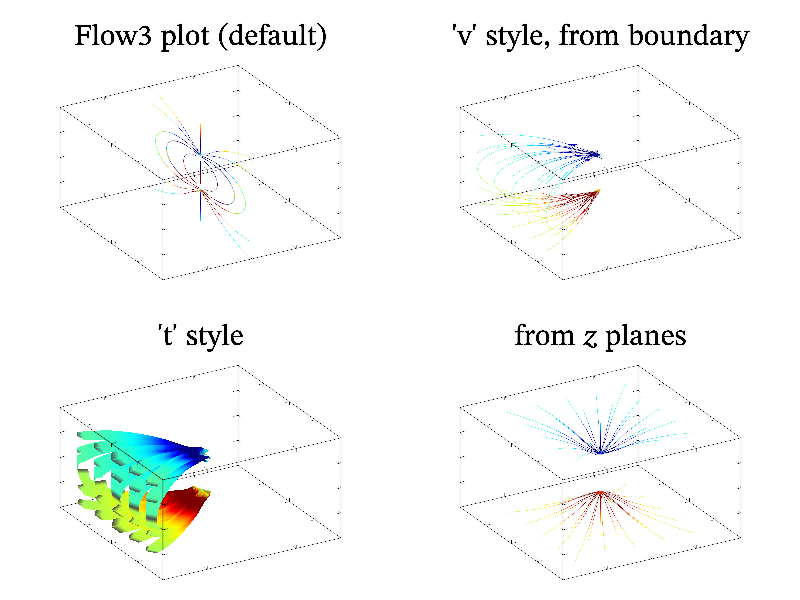
Next: fonts sample, Previous: flow3 sample, Up: All samples [Contents][Index]
Example of fog.
MGL code:
call 'prepare2d' title 'Fog sample':rotate 50 60:light on:fog 1 box:surf a:cont a 'y'
C++ code:
void smgl_fog(mglGraph *gr)
{
mglData a; mgls_prepare2d(&a);
if(big!=3) gr->Title("Fog sample");
gr->Light(true); gr->Rotate(50,60); gr->Fog(1); gr->Box();
gr->Surf(a); gr->Cont(a,"y");
}
Next: grad sample, Previous: fog sample, Up: All samples [Contents][Index]
Example of font typefaces.
MGL code:
define d 0.25 loadfont 'STIX':text 0 1.1 'default font (STIX)' loadfont 'adventor':text 0 1.1-d 'adventor font' loadfont 'bonum':text 0 1.1-2*d 'bonum font' loadfont 'chorus':text 0 1.1-3*d 'chorus font' loadfont 'cursor':text 0 1.1-4*d 'cursor font' loadfont 'heros':text 0 1.1-5*d 'heros font' loadfont 'heroscn':text 0 1.1-6*d 'heroscn font' loadfont 'pagella':text 0 1.1-7*d 'pagella font' loadfont 'schola':text 0 1.1-8*d 'schola font' loadfont 'termes':text 0 1.1-9*d 'termes font' loadfont ''
C++ code:
void smgl_fonts(mglGraph *gr) // font typefaces
{
double h=1.1, d=0.25;
gr->LoadFont("STIX"); gr->Puts(mglPoint(0,h), "default font (STIX)");
gr->LoadFont("adventor"); gr->Puts(mglPoint(0,h-d), "adventor font");
gr->LoadFont("bonum"); gr->Puts(mglPoint(0,h-2*d), "bonum font");
gr->LoadFont("chorus"); gr->Puts(mglPoint(0,h-3*d), "chorus font");
gr->LoadFont("cursor"); gr->Puts(mglPoint(0,h-4*d), "cursor font");
gr->LoadFont("heros"); gr->Puts(mglPoint(0,h-5*d), "heros font");
gr->LoadFont("heroscn"); gr->Puts(mglPoint(0,h-6*d), "heroscn font");
gr->LoadFont("pagella"); gr->Puts(mglPoint(0,h-7*d), "pagella font");
gr->LoadFont("schola"); gr->Puts(mglPoint(0,h-8*d), "schola font");
gr->LoadFont("termes"); gr->Puts(mglPoint(0,h-9*d), "termes font");
gr->LoadFont("");
}
Next: hist sample, Previous: fonts sample, Up: All samples [Contents][Index]
Function grad draw gradient lines for matrix.
MGL code:
call 'prepare2d'
subplot 1 1 0 '':title 'Grad plot':box:grad a:dens a '{u8}w{q8}'
C++ code:
void smgl_grad(mglGraph *gr)
{
mglData a; mgls_prepare2d(&a);
if(big!=3) {gr->SubPlot(1,1,0,""); gr->Title("Grad plot");}
gr->Box(); gr->Grad(a); gr->Dens(a,"{u8}w{q8}");
}
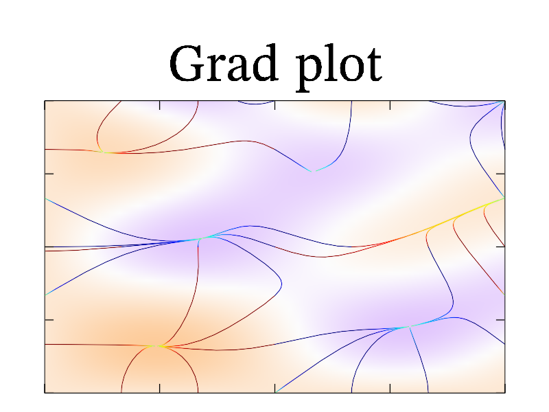
Next: icon sample, Previous: grad sample, Up: All samples [Contents][Index]
Example of hist (histogram).
MGL code:
new x 10000 '2*rnd-1':new y 10000 '2*rnd-1':copy z exp(-6*(x^2+y^2))
hist xx x z:norm xx 0 1:hist yy y z:norm yy 0 1
multiplot 3 3 3 2 2 '':ranges -1 1 -1 1 0 1:box:dots x y z 'wyrRk'
multiplot 3 3 0 2 1 '':ranges -1 1 0 1:box:bars xx
multiplot 3 3 5 1 2 '':ranges 0 1 -1 1:box:barh yy
subplot 3 3 2:text 0.5 0.5 'Hist and\n{}MultiPlot\n{}sample' 'a' -3
C++ code:
void smgl_hist(mglGraph *gr)
{
mglData x(10000), y(10000), z(10000); gr->Fill(x,"2*rnd-1"); gr->Fill(y,"2*rnd-1"); gr->Fill(z,"exp(-6*(v^2+w^2))",x,y);
mglData xx=gr->Hist(x,z), yy=gr->Hist(y,z); xx.Norm(0,1); yy.Norm(0,1);
gr->MultiPlot(3,3,3,2,2,""); gr->SetRanges(-1,1,-1,1,0,1); gr->Box(); gr->Dots(x,y,z,"wyrRk");
gr->MultiPlot(3,3,0,2,1,""); gr->SetRanges(-1,1,0,1); gr->Box(); gr->Bars(xx);
gr->MultiPlot(3,3,5,1,2,""); gr->SetRanges(0,1,-1,1); gr->Box(); gr->Barh(yy);
gr->SubPlot(3,3,2); gr->Puts(mglPoint(0.5,0.5),"Hist and\nMultiPlot\nsample","a",-3);
}
Next: ifs2d sample, Previous: hist sample, Up: All samples [Contents][Index]
Default UDAV and mgllab icon.
MGL code:
setsize 200 200 zrange 0 2 define $s 0.8 new x 200 '$s*(x+1)/2*sin(2*pi*x)' new y 200 '$s*(x+1)/2*cos(2*pi*x)' new z 200 '$s*(2-(x+1))+0.1' new r 200 '0.02+0.07*(x+1)' subplot 1 1 0 '#' fsurf 'v*cos(2*pi*u)' 'v*sin(2*pi*u)-0.05' 'v/2' 'Yyyww' light on rotate 65 80 tube x y z+0.15 r define $r 0.13 fsurf '0+$r*cos(2*pi*u)*cos(2*pi*v)' '0.03+$r*cos(2*pi*u)*sin(2*pi*v)' '2*$s+0.25+$r*sin(2*pi*u)' 'r' define $r 0.155 fsurf '$r*cos(2*pi*u)*cos(2*pi*v)' '$s+$r*cos(2*pi*u)*sin(2*pi*v)' '0.25+$r*sin(2*pi*u)' 'b'
C++ code:
void smgl_icon(mglGraph *gr)
{
gr->SetSize(200,200); gr->SetRange('z',0,2);
mglData x(200); gr->Fill(x,"0.8*(x+1)/2*sin(2*pi*x)");
mglData y(200); gr->Fill(y,"0.8*(x+1)/2*cos(2*pi*x)");
mglData z(200); gr->Fill(z,"0.8*(2-(x+1))+0.25");
mglData r(200); gr->Fill(r,"0.02+0.07*(x+1)");
gr->SubPlot(1,1,0,"#");
gr->FSurf("v*cos(2*pi*u)","v*sin(2*pi*u)-0.05","v/2","Yyyww");
gr->Light(true); gr->Rotate(65,80); gr->Tube(x,y,z,r);
gr->FSurf("0.13*cos(2*pi*u)*cos(2*pi*v)","0.03+0.13*cos(2*pi*u)*sin(2*pi*v)","1.85+0.13*sin(2*pi*u)","r");
gr->FSurf("0.155*cos(2*pi*u)*cos(2*pi*v)","0.8+0.155*cos(2*pi*u)*sin(2*pi*v)","0.25+0.155*sin(2*pi*u)","b");
}
Next: ifs3d sample, Previous: icon sample, Up: All samples [Contents][Index]
Function ifs2d generate points for fractals using iterated function system in 2d case.
MGL code:
list A [0.33,0,0,0.33,0,0,0.2] [0.33,0,0,0.33,0.67,0,0.2] [0.33,0,0,0.33,0.33,0.33,0.2]\ [0.33,0,0,0.33,0,0.67,0.2] [0.33,0,0,0.33,0.67,0.67,0.2] ifs2d fx fy A 100000 subplot 1 1 0 '<_':title 'IFS 2d sample' ranges fx fy:axis plot fx fy 'r#o ';size 0.05
C++ code:
void smgl_ifs2d(mglGraph *gr)
{
mglData A;
A.SetList(35, 0.33,0.,0.,0.33,0.,0.,0.2, 0.33,0.,0.,0.33,0.67,0.,0.2, 0.33,0.,0.,0.33,0.33,0.33,0.2, 0.33,0.,0.,0.33,0.,0.67,0.2, 0.33,0.,0.,0.33,0.67,0.67,0.2);
A.Rearrange(7);
mglData f(mglIFS2d(A,100000));
gr->SubPlot(1,1,0,"<_");
if(big!=3) gr->Title("IFS 2d sample");
gr->SetRanges(f.SubData(0), f.SubData(1));
gr->Axis(); gr->Plot(f.SubData(0), f.SubData(1),"r#o ","size 0.05");
}

Next: indirect sample, Previous: ifs2d sample, Up: All samples [Contents][Index]
Function ifs3d generate points for fractals using iterated function system in 3d case.
MGL code:
list A [0,0,0,0,.18,0,0,0,0,0,0,0,.01] [.85,0,0,0,.85,.1,0,-0.1,0.85,0,1.6,0,.85]\ [.2,-.2,0,.2,.2,0,0,0,0.3,0,0.8,0,.07] [-.2,.2,0,.2,.2,0,0,0,0.3,0,0.8,0,.07] ifs3d f A 100000 title 'IFS 3d sample':rotate 50 60 ranges f(0) f(1) f(2):axis:box dots f(0) f(1) f(2) 'G#o';size 0.05
C++ code:
void smgl_ifs3d(mglGraph *gr)
{
mglData A;
A.SetList(52, 0.,0.,0.,0.,.18,0.,0.,0.,0.,0.,0.,0.,.01, .85,0.,0.,0.,.85,.1,0.,-0.1,0.85,0.,1.6,0.,.85,
.2,-.2,0.,.2,.2,0.,0.,0.,0.3,0.,0.8,0.,.07, -.2,.2,0.,.2,.2,0.,0.,0.,0.3,0.,0.8,0.,.07);
A.Rearrange(13);
mglData f(mglIFS3d(A,100000));
if(big!=3) gr->Title("IFS 3d sample");
gr->SetRanges(f.SubData(0), f.SubData(1), f.SubData(2));
gr->Rotate(50,60); gr->Axis(); gr->Box();
gr->Dots(f.SubData(0), f.SubData(1), f.SubData(2),"G#o","size 0.05");
}
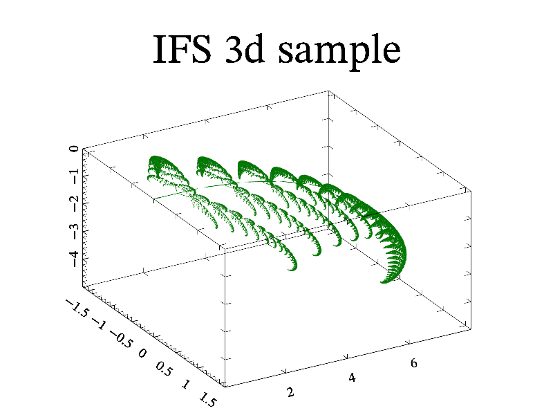
Next: inplot sample, Previous: ifs3d sample, Up: All samples [Contents][Index]
Comparison of subdata vs evaluate/
MGL code:
subplot 1 1 0 '':title 'SubData vs Evaluate' new in 9 'x^3/1.1':plot in 'ko ':box new arg 99 '4*x+4' evaluate e in arg off:plot e 'b.'; legend 'Evaluate' subdata s in arg:plot s 'r.';legend 'SubData' legend 2
C++ code:
void smgl_indirect(mglGraph *gr)
{
gr->SubPlot(1,1,0,""); gr->Title("SubData vs Evaluate");
mglData in(9), arg(99), e, s;
gr->Fill(in,"x^3/1.1"); gr->Fill(arg,"4*x+4");
gr->Plot(in,"ko "); gr->Box();
e = in.Evaluate(arg,false); gr->Plot(e,"b.","legend 'Evaluate'");
s = in.SubData(arg); gr->Plot(s,"r.","legend 'SubData'");
gr->Legend(2);
}
Next: iris sample, Previous: indirect sample, Up: All samples [Contents][Index]
Example of inplot, multiplot, columnplot, gridplot, shearplot, stickplot.
MGL code:
subplot 3 2 0:title 'StickPlot' stickplot 3 0 20 30:box 'r':text 0 0 0 '0' 'r' stickplot 3 1 20 30:box 'g':text 0 0 0 '1' 'g' stickplot 3 2 20 30:box 'b':text 0 9 0 '2' 'b' subplot 3 2 3 '':title 'ColumnPlot' columnplot 3 0:box 'r':text 0 0 '0' 'r' columnplot 3 1:box 'g':text 0 0 '1' 'g' columnplot 3 2:box 'b':text 0 0 '2' 'b' subplot 3 2 4 '':title 'GridPlot' gridplot 2 2 0:box 'r':text 0 0 '0' 'r' gridplot 2 2 1:box 'g':text 0 0 '1' 'g' gridplot 2 2 2:box 'b':text 0 0 '2' 'b' gridplot 2 2 3:box 'm':text 0 0 '3' 'm' subplot 3 2 5 '':title 'InPlot':box inplot 0.4 1 0.6 1 on:box 'r' multiplot 3 2 1 2 1 '':title 'MultiPlot and ShearPlot':box shearplot 3 0 0.2 0.1:box 'r':text 0 0 '0' 'r' shearplot 3 1 0.2 0.1:box 'g':text 0 0 '1' 'g' shearplot 3 2 0.2 0.1:box 'b':text 0 0 '2' 'b'
C++ code:
void smgl_inplot(mglGraph *gr)
{
gr->SubPlot(3,2,0); gr->Title("StickPlot");
gr->StickPlot(3, 0, 20, 30); gr->Box("r"); gr->Puts(mglPoint(0),"0","r");
gr->StickPlot(3, 1, 20, 30); gr->Box("g"); gr->Puts(mglPoint(0),"1","g");
gr->StickPlot(3, 2, 20, 30); gr->Box("b"); gr->Puts(mglPoint(0),"2","b");
gr->SubPlot(3,2,3,""); gr->Title("ColumnPlot");
gr->ColumnPlot(3, 0); gr->Box("r"); gr->Puts(mglPoint(0),"0","r");
gr->ColumnPlot(3, 1); gr->Box("g"); gr->Puts(mglPoint(0),"1","g");
gr->ColumnPlot(3, 2); gr->Box("b"); gr->Puts(mglPoint(0),"2","b");
gr->SubPlot(3,2,4,""); gr->Title("GridPlot");
gr->GridPlot(2, 2, 0); gr->Box("r"); gr->Puts(mglPoint(0),"0","r");
gr->GridPlot(2, 2, 1); gr->Box("g"); gr->Puts(mglPoint(0),"1","g");
gr->GridPlot(2, 2, 2); gr->Box("b"); gr->Puts(mglPoint(0),"2","b");
gr->GridPlot(2, 2, 3); gr->Box("m"); gr->Puts(mglPoint(0),"3","m");
gr->SubPlot(3,2,5,""); gr->Title("InPlot"); gr->Box();
gr->InPlot(0.4, 1, 0.6, 1, true); gr->Box("r");
gr->MultiPlot(3,2,1, 2, 1,""); gr->Title("MultiPlot and ShearPlot"); gr->Box();
gr->ShearPlot(3, 0, 0.2, 0.1); gr->Box("r"); gr->Puts(mglPoint(0),"0","r");
gr->ShearPlot(3, 1, 0.2, 0.1); gr->Box("g"); gr->Puts(mglPoint(0),"1","g");
gr->ShearPlot(3, 2, 0.2, 0.1); gr->Box("b"); gr->Puts(mglPoint(0),"2","b");
}
Next: keep sample, Previous: inplot sample, Up: All samples [Contents][Index]
Function iris draw Iris plot for columns of data array.
MGL code:
read a 'iris.dat' crop a 0 4 'x':rearrange a a.nx 50 subplot 1 1 0 '':title 'Iris plot' iris a 'sepal\n length;sepal\n width;petal\n length;petal\n width' '. ';value -1.5;size -2
C++ code:
void smgl_iris(mglGraph *gr)
{
mglData a("iris.dat"); a.Crop(0,4,'x'); a.Rearrange(4,50);
gr->SubPlot(1,1,0,"");
if(big!=3) gr->Title("Iris sample");
gr->Iris(a, "sepal\nlength;sepal\nwidth;petal\nlength;petal\nwidth", ". ", "value -1.5;size -2");
}

Next: label sample, Previous: iris sample, Up: All samples [Contents][Index]
Function keep conserve initial phase along specified direction(s).
MGL code:
yrange 0 pi new !a 100 300 'exp(-6*x^2+10i*(x+y^2))'subplot 2 1 0 '':box dens real(a) 'BbwrR' text 1.1 0.5 ' o' 'a'keep a 'y' 50 subplot 2 1 1 '':box dens real(a) 'BbwrR'
C++ code:
void smgl_keep(mglGraph *gr)
{
gr->SetRange('y',0,M_PI);
mglDataC a(100,300); gr->Fill(a,"exp(-6*x^2+10i*(x+y^2))");
gr->SubPlot(2,1,0,""); gr->Box();
gr->Dens(a.Real(),"BbwrR");
gr->Puts(1.1,0.5,"\\to","a");
a.Keep("y",50);
gr->SubPlot(2,1,1,""); gr->Box();
gr->Dens(a.Real(),"BbwrR");
}
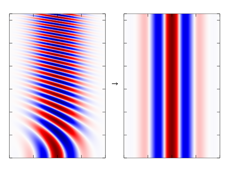
Next: lamerey sample, Previous: keep sample, Up: All samples [Contents][Index]
Function label print text at data points. The string may contain ‘%x’, ‘%y’, ‘%z’ for x-, y-, z-coordinates of points, ‘%n’ for point index.
MGL code:
new ys 10 '0.2*rnd-0.8*sin(pi*x)' subplot 1 1 0 '':title 'Label plot':box:plot ys ' *':label ys 'y=%y'
C++ code:
void smgl_label(mglGraph *gr)
{
mglData ys(10); ys.Modify("0.8*sin(pi*2*x)+0.2*rnd");
if(big!=3) { gr->SubPlot(1,1,0,""); gr->Title("Label plot"); }
gr->Box(); gr->Plot(ys," *"); gr->Label(ys,"y=%y");
}
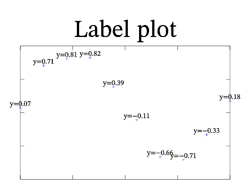
Next: legend sample, Previous: label sample, Up: All samples [Contents][Index]
Function lamerey draw Lamerey diagram.
MGL code:
subplot 1 1 0 '<_':title 'Lamerey sample'
axis:xlabel '\i x':ylabel '\bar{\i x} = 2 \i{x}'
fplot 'x' 'k='
fplot '2*x' 'b'
lamerey 0.00097 '2*x' 'rv~';size 2
lamerey -0.00097 '2*x' 'rv~';size 2
C++ code:
void smgl_lamerey(mglGraph *gr)
{
gr->SubPlot(1,1,0,"<_");
if(big!=3) gr->Title("Lamerey sample");
gr->Axis(); gr->Label('x',"\\i x"); gr->Label('y',"\\bar{\\i x} = 2 \\i{x}");
gr->FPlot("x","k="); gr->FPlot("2*x","b");
gr->Lamerey( 0.00097,"2*x","rv~");
gr->Lamerey(-0.00097,"2*x","rv~");
}
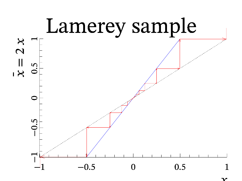
Next: light sample, Previous: lamerey sample, Up: All samples [Contents][Index]
Example of legend styles.
MGL code:
addlegend 'sin(\pi {x^2})' 'b':addlegend 'sin(\pi x)' 'g*'
addlegend 'sin(\pi \sqrt{x})' 'rd':addlegend 'jsut text' ' ':addlegend 'no indent for this' ''
subplot 2 2 0 '':title 'Legend (default)':box:legend
legend 1 0.5 '^':text 0.49 0.88 'Style "\^"' 'A:L'
legend 3 'A#':text 0.75 0.65 'Absolute position' 'A'
subplot 2 2 2 '':title 'coloring':box:legend 0 'r#':legend 1 'Wb#':legend 2 'ygr#'
subplot 2 2 3 '':title 'manual position':box
legend 0.5 1:text 0.5 0.5 'at x=0.5, y=1' 'a'
legend 1 '#-':text 0.75 0.25 'Horizontal legend' 'a'
C++ code:
void smgl_legend(mglGraph *gr)
{
gr->AddLegend("sin(\\pi {x^2})","b");
gr->AddLegend("sin(\\pi x)","g*");
gr->AddLegend("sin(\\pi \\sqrt{x})","rd");
gr->AddLegend("just text"," ");
gr->AddLegend("no indent for this","");
if(big!=3) {gr->SubPlot(2,2,0,""); gr->Title("Legend (default)");}
gr->Box(); gr->Legend();
if(big==3) return;
gr->Legend(1,0.5,"^"); gr->Puts(0.49, 0.88, "Style '\\^'","A:L");
gr->Legend(3,"A#");
gr->Puts(mglPoint(0.75,0.65),"Absolute position","A");
gr->SubPlot(2,2,2,""); gr->Title("coloring"); gr->Box();
gr->Legend(0,"r#"); gr->Legend(1,"Wb#"); gr->Legend(2,"ygr#");
gr->SubPlot(2,2,3,""); gr->Title("manual position"); gr->Box();
gr->Legend(0.5,1);
gr->Puts(mglPoint(0.5,0.5),"at x=0.5, y=1","a");
gr->Legend(1,"#-");
gr->Puts(mglPoint(0.75,0.25),"Horizontal legend","a");
}
Next: lines sample, Previous: legend sample, Up: All samples [Contents][Index]
Example of light with different types.
MGL code:
light on:attachlight on call 'prepare2d' subplot 2 2 0:title 'Default':rotate 50 60:box:surf a line -1 -0.7 1.7 -1 -0.7 0.7 'BA' subplot 2 2 1:title 'Local':rotate 50 60 light 0 1 0 1 -2 -1 -1 line 1 0 1 -1 -1 0 'BAO':box:surf a subplot 2 2 2:title 'no diffuse':rotate 50 60 diffuse 0 line 1 0 1 -1 -1 0 'BAO':box:surf a subplot 2 2 3:title 'diffusive only':rotate 50 60 diffuse 0.5:light 0 1 0 1 -2 -1 -1 'w' 0 line 1 0 1 -1 -1 0 'BAO':box:surf a
C++ code:
void smgl_light(mglGraph *gr) // local light sources
{
mglData a; mgls_prepare2d(&a);
gr->Light(true); gr->AttachLight(true);
if(big==3)
{ gr->Rotate(50,60); gr->Box(); gr->Surf(a); return; }
gr->SubPlot(2,2,0); gr->Title("Default"); gr->Rotate(50,60);
gr->Line(mglPoint(-1,-0.7,1.7),mglPoint(-1,-0.7,0.7),"BA"); gr->Box(); gr->Surf(a);
gr->SubPlot(2,2,1); gr->Title("Local"); gr->Rotate(50,60);
gr->AddLight(0,mglPoint(1,0,1),mglPoint(-2,-1,-1));
gr->Line(mglPoint(1,0,1),mglPoint(-1,-1,0),"BAO"); gr->Box(); gr->Surf(a);
gr->SubPlot(2,2,2); gr->Title("no diffuse"); gr->Rotate(50,60);
gr->SetDiffuse(0);
gr->Line(mglPoint(1,0,1),mglPoint(-1,-1,0),"BAO"); gr->Box(); gr->Surf(a);
gr->SubPlot(2,2,3); gr->Title("diffusive only"); gr->Rotate(50,60);
gr->SetDiffuse(0.5);
gr->AddLight(0,mglPoint(1,0,1),mglPoint(-2,-1,-1),'w',0);
gr->Line(mglPoint(1,0,1),mglPoint(-1,-1,0),"BAO"); gr->Box(); gr->Surf(a);
}
Next: loglog sample, Previous: light sample, Up: All samples [Contents][Index]
Function lines draw a set of lines.
MGL code:
subplot 1 1 0 '':title 'Lines plot' new x1 11 '0.3*cos(pi*i/5)' new y1 11 '0.3*sin(pi*i/5)' new x2 11 '0.7*cos(pi*i/5)' new y2 11 '0.7*sin(pi*i/5)' plot x1 y1 lines x1 y1 x2 y2 '_A'
C++ code:
void smgl_lines(mglGraph *gr)
{
mglData x1(11),y1(11),x2(11),y2(11);
for(long i=0;i<11;i++)
{
x1.a[i] = 0.3*cos(M_PI*i/5);
y1.a[i] = 0.3*sin(M_PI*i/5);
x2.a[i] = 0.7*cos(M_PI*i/5);
y2.a[i] = 0.7*sin(M_PI*i/5);
}
if(big!=3) {gr->SubPlot(1,1,0,""); gr->Title("Lines plot");}
gr->Plot(x1,y1);
gr->Lines(x1,y1,x2,y2,"_A");
}
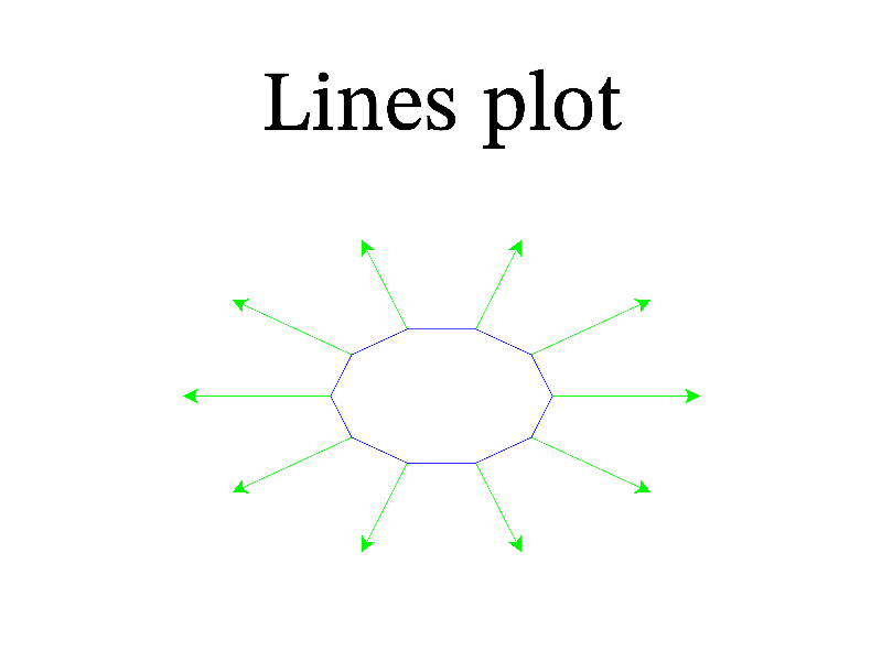
Next: map sample, Previous: lines sample, Up: All samples [Contents][Index]
Example of log- and log-log- axis labels.
MGL code:
subplot 2 2 0 '<_':title 'Semi-log axis':ranges 0.01 100 -1 1:axis 'lg(x)' '' ''
axis:grid 'xy' 'g':fplot 'sin(1/x)':xlabel 'x' 0:ylabel 'y = sin 1/x' 0
subplot 2 2 1 '<_':title 'Log-log axis':ranges 0.01 100 0.1 100:axis 'lg(x)' 'lg(y)' ''
axis:grid '!' 'h=':grid:fplot 'sqrt(1+x^2)'
xlabel 'x' 0:ylabel 'y = \sqrt{1+x^2}' 0
subplot 2 2 2 '<_':title 'Minus-log axis':ranges -100 -0.01 -100 -0.1:axis '-lg(-x)' '-lg(-y)' ''
axis:fplot '-sqrt(1+x^2)':xlabel 'x' 0:ylabel 'y = -\sqrt{1+x^2}' 0
subplot 2 2 3 '<_':title 'Log-ticks':ranges 0.01 100 0 100:axis 'sqrt(x)' '' ''
axis:fplot 'x':xlabel 'x' 1:ylabel 'y = x' 0
C++ code:
void smgl_loglog(mglGraph *gr) // log-log axis
{
gr->SubPlot(2,2,0,"<_"); gr->Title("Semi-log axis"); gr->SetRanges(0.01,100,-1,1); gr->SetFunc("lg(x)","");
gr->Axis(); gr->Grid("xy","g"); gr->FPlot("sin(1/x)"); gr->Label('x',"x",0); gr->Label('y', "y = sin 1/x",0);
gr->SubPlot(2,2,1,"<_"); gr->Title("Log-log axis"); gr->SetRanges(0.01,100,0.1,100); gr->SetFunc("lg(x)","lg(y)");
gr->Axis(); gr->Grid("!","h="); gr->Grid(); gr->FPlot("sqrt(1+x^2)"); gr->Label('x',"x",0); gr->Label('y', "y = \\sqrt{1+x^2}",0);
gr->SubPlot(2,2,2,"<_"); gr->Title("Minus-log axis"); gr->SetRanges(-100,-0.01,-100,-0.1); gr->SetFunc("-lg(-x)","-lg(-y)");
gr->Axis(); gr->FPlot("-sqrt(1+x^2)"); gr->Label('x',"x",0); gr->Label('y', "y = -\\sqrt{1+x^2}",0);
gr->SubPlot(2,2,3,"<_"); gr->Title("Log-ticks"); gr->SetRanges(0.1,100,0,100); gr->SetFunc("sqrt(x)","");
gr->Axis(); gr->FPlot("x"); gr->Label('x',"x",1); gr->Label('y', "y = x",0);
}
Next: mark sample, Previous: loglog sample, Up: All samples [Contents][Index]
Example of map.
MGL code:
new a 50 40 'x':new b 50 40 'y':zrange -2 2:text 0 0 '\to'
subplot 2 1 0:text 0 1.1 '\{x, y\}' '' -2:box:map a b 'brgk'
subplot 2 1 1:text 0 1.1 '\{\frac{x^3+y^3}{2}, \frac{x-y}{2}\}' '' -2
box:fill a '(x^3+y^3)/2':fill b '(x-y)/2':map a b 'brgk'
C++ code:
void smgl_map(mglGraph *gr) // example of mapping
{
mglData a(50, 40), b(50, 40);
gr->Puts(mglPoint(0, 0), "\\to", ":C", -1.4);
gr->SetRanges(-1,1,-1,1,-2,2);
gr->SubPlot(2, 1, 0);
gr->Fill(a,"x"); gr->Fill(b,"y");
gr->Puts(mglPoint(0, 1.1), "\\{x, y\\}", ":C", -2); gr->Box();
gr->Map(a, b, "brgk");
gr->SubPlot(2, 1, 1);
gr->Fill(a,"(x^3+y^3)/2"); gr->Fill(b,"(x-y)/2");
gr->Puts(mglPoint(0, 1.1), "\\{\\frac{x^3+y^3}{2}, \\frac{x-y}{2}\\}", ":C", -2);
gr->Box();
gr->Map(a, b, "brgk");
}
Next: mask sample, Previous: map sample, Up: All samples [Contents][Index]
Example of mark.
MGL code:
call 'prepare1d' subplot 1 1 0 '':title 'Mark plot (default)':box:mark y y1 's'
C++ code:
void smgl_mark(mglGraph *gr)
{
mglData y,y1; mgls_prepare1d(&y,&y1);
if(big!=3) { gr->SubPlot(1,1,0,""); gr->Title("Mark plot (default)"); }
gr->Box(); gr->Mark(y,y1,"s");
}
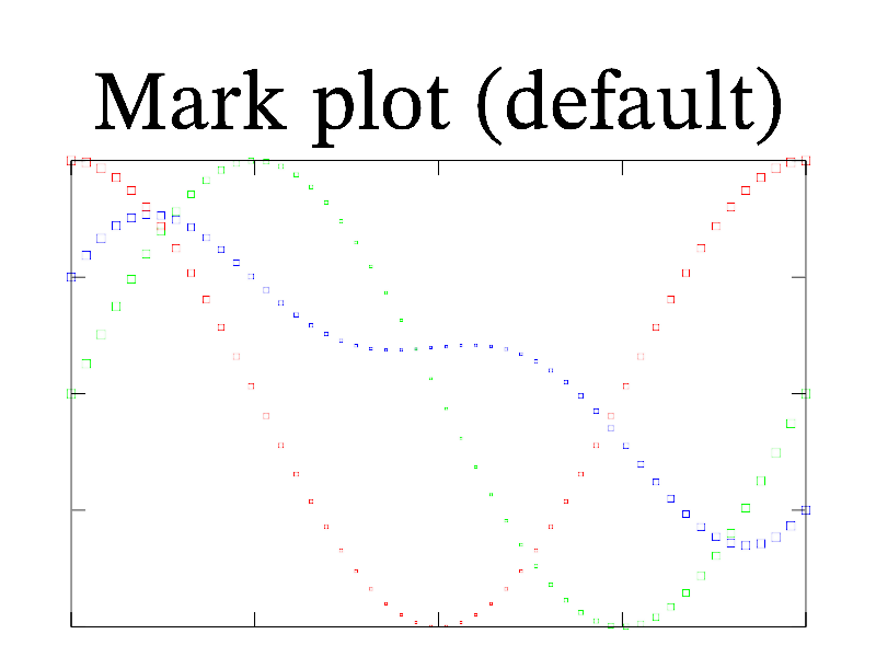
Next: mesh sample, Previous: mark sample, Up: All samples [Contents][Index]
Example of mask kinds.
MGL code:
new a 10 10 'x' subplot 5 4 0 '':title '"-" mask':dens a '3-' subplot 5 4 1 '':title '"+" mask':dens a '3+' subplot 5 4 2 '':title '"=" mask':dens a '3=' subplot 5 4 3 '':title '";" mask':dens a '3;' subplot 5 4 4 '':title '";I" mask':dens a '3;I' subplot 5 4 5 '':title '"o" mask':dens a '3o' subplot 5 4 6 '':title '"O" mask':dens a '3O' subplot 5 4 7 '':title '"s" mask':dens a '3s' subplot 5 4 8 '':title '"S" mask':dens a '3S' subplot 5 4 9 '':title '";/" mask':dens a '3;/' subplot 5 4 10 '':title '"~" mask':dens a '3~' subplot 5 4 11 '':title '"<" mask':dens a '3<' subplot 5 4 12 '':title '">" mask':dens a '3>' subplot 5 4 13 '':title '"j" mask':dens a '3j' subplot 5 4 14 '':title '"-;\" mask':dens a '3\;' subplot 5 4 15 '':title '"d" mask':dens a '3d' subplot 5 4 16 '':title '"D" mask':dens a '3D' subplot 5 4 17 '':title '"*" mask':dens a '3*' subplot 5 4 18 '':title '"\^" mask':dens a '3^' subplot 5 4 19 '':title 'manual mask' mask '+' '24242424FF0101FF':dens a '3+'
C++ code:
void smgl_mask(mglGraph *gr)
{
mglData a(10,10); a.Fill(-1,1);
gr->SubPlot(5,4,0,""); gr->Title("'-' mask"); gr->Dens(a,"3-");
gr->SubPlot(5,4,1,""); gr->Title("'+' mask"); gr->Dens(a,"3+");
gr->SubPlot(5,4,2,""); gr->Title("'=' mask"); gr->Dens(a,"3=");
gr->SubPlot(5,4,3,""); gr->Title("';' mask"); gr->Dens(a,"3;");
gr->SubPlot(5,4,4,""); gr->Title("';I' mask"); gr->Dens(a,"3;I");
gr->SubPlot(5,4,5,""); gr->Title("'o' mask"); gr->Dens(a,"3o");
gr->SubPlot(5,4,6,""); gr->Title("'O' mask"); gr->Dens(a,"3O");
gr->SubPlot(5,4,7,""); gr->Title("'s' mask"); gr->Dens(a,"3s");
gr->SubPlot(5,4,8,""); gr->Title("'S' mask"); gr->Dens(a,"3S");
gr->SubPlot(5,4,9,""); gr->Title("';/' mask"); gr->Dens(a,"3;/");
gr->SubPlot(5,4,10,""); gr->Title("'~' mask"); gr->Dens(a,"3~");
gr->SubPlot(5,4,11,""); gr->Title("'<' mask"); gr->Dens(a,"3<");
gr->SubPlot(5,4,12,""); gr->Title("'>' mask"); gr->Dens(a,"3>");
gr->SubPlot(5,4,13,""); gr->Title("'j' mask"); gr->Dens(a,"3j");
gr->SubPlot(5,4,14,""); gr->Title("';\\\\' mask"); gr->Dens(a,"3;\\");
gr->SubPlot(5,4,15,""); gr->Title("'d' mask"); gr->Dens(a,"3d");
gr->SubPlot(5,4,16,""); gr->Title("'D' mask"); gr->Dens(a,"3D");
gr->SubPlot(5,4,17,""); gr->Title("'*' mask"); gr->Dens(a,"3*");
gr->SubPlot(5,4,18,""); gr->Title("'\\^' mask"); gr->Dens(a,"3^");
gr->SubPlot(5,4,19,""); gr->Title("manual mask");
gr->SetMask('+', "24242424FF0101FF"); gr->Dens(a,"3+");
}
Next: minmax sample, Previous: mask sample, Up: All samples [Contents][Index]
Function mesh draw wired surface. You can use meshnum for changing number of lines to be drawn.
MGL code:
call 'prepare2d' title 'Mesh plot':rotate 50 60:box:mesh a
C++ code:
void smgl_mesh(mglGraph *gr)
{
mglData a; mgls_prepare2d(&a);
if(big!=3) gr->Title("Mesh plot");
gr->Rotate(50,60); gr->Box(); gr->Mesh(a);
}
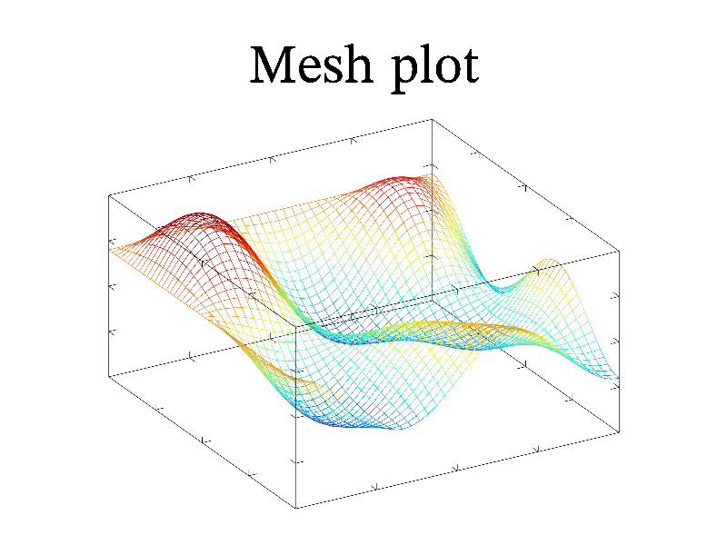
Next: mirror sample, Previous: mesh sample, Up: All samples [Contents][Index]
Function minmax get position of local minimums and maximums.
MGL code:
define $p 30 new h 300 300 '-sqrt(1-x^2-y^2)*(3*x*y^2*$p-x^3*$p+6*y)/(3*sqrt(2))+x*y+(y^2+x^2)*$p/3 -7*(y^2+x^2)^2*$p/24+y^2+3*x^2' minmax e h subplot 1 1 0 '':title 'MinMax sample' crange h:dens h:box fplot 'sin(2*pi*t)' 'cos(2*pi*t)' '0' 'k' plot e(0)*2-1 e(1)*2-1 '. c'
C++ code:
void smgl_minmax(mglGraph *gr) // test minmax
{
mglData h(300,300);
gr->Fill(h,"-sqrt(1-x^2-y^2)*(3*x*y^2*30-x^3*30+6*y)/(3*sqrt(2))+x*y+(y^2+x^2)*10 -7*(y^2+x^2)^2*30/24+y^2+3*x^2");
mglData e=h.MinMax();
if(big!=3) { gr->SubPlot(1,1,0,""); gr->Title("MinMax sample"); }
gr->SetRange('c',h); gr->Dens(h); gr->Box();
gr->FPlot("sin(2*pi*t)","cos(2*pi*t)","0","k");
e*=2; e-=1;
gr->Plot(e(0),e(1),". c");
}
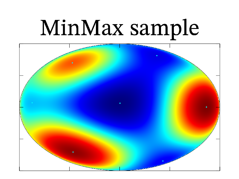
Next: molecule sample, Previous: minmax sample, Up: All samples [Contents][Index]
Example of using options.
MGL code:
new a 31 41 '-pi*x*exp(-(y+1)^2-4*x^2)' subplot 2 2 0:title 'Options for coordinates':alpha on:light on:rotate 40 60:box surf a 'r';yrange 0 1:surf a 'b';yrange 0 -1 subplot 2 2 1:title 'Option "meshnum"':rotate 40 60:box mesh a 'r'; yrange 0 1:mesh a 'b';yrange 0 -1; meshnum 5 subplot 2 2 2:title 'Option "alpha"':rotate 40 60:box surf a 'r';yrange 0 1; alpha 0.7:surf a 'b';yrange 0 -1; alpha 0.3 subplot 2 2 3 '<_':title 'Option "legend"' fplot 'x^3' 'r'; legend 'y = x^3':fplot 'cos(pi*x)' 'b'; legend 'y = cos \pi x' box:axis:legend 2
C++ code:
void smgl_mirror(mglGraph *gr) // flag #
{
mglData a(31,41);
gr->Fill(a,"-pi*x*exp(-(y+1)^2-4*x^2)");
if(big!=3) { gr->SubPlot(2,2,0); gr->Title("Options for coordinates"); }
gr->Alpha(true); gr->Light(true);
gr->Rotate(40,60); gr->Box();
gr->Surf(a,"r","yrange 0 1"); gr->Surf(a,"b","yrange 0 -1");
if(big==3) return;
gr->SubPlot(2,2,1); gr->Title("Option 'meshnum'");
gr->Rotate(40,60); gr->Box();
gr->Mesh(a,"r","yrange 0 1"); gr->Mesh(a,"b","yrange 0 -1; meshnum 5");
gr->SubPlot(2,2,2); gr->Title("Option 'alpha'");
gr->Rotate(40,60); gr->Box();
gr->Surf(a,"r","yrange 0 1; alpha 0.7"); gr->Surf(a,"b","yrange 0 -1; alpha 0.3");
gr->SubPlot(2,2,3,"<_"); gr->Title("Option 'legend'");
gr->FPlot("x^3","r","legend 'y = x^3'"); gr->FPlot("cos(pi*x)","b","legend 'y = cos \\pi x'");
gr->Box(); gr->Axis(); gr->Legend(2,"");
}
Next: ode sample, Previous: mirror sample, Up: All samples [Contents][Index]
Example of drawing molecules.
MGL code:
alpha on:light on
subplot 2 2 0 '':title 'Methane, CH_4':rotate 60 120
sphere 0 0 0 0.25 'k':drop 0 0 0 0 0 1 0.35 'h' 1 2:sphere 0 0 0.7 0.25 'g'
drop 0 0 0 -0.94 0 -0.33 0.35 'h' 1 2:sphere -0.66 0 -0.23 0.25 'g'
drop 0 0 0 0.47 0.82 -0.33 0.35 'h' 1 2:sphere 0.33 0.57 -0.23 0.25 'g'
drop 0 0 0 0.47 -0.82 -0.33 0.35 'h' 1 2:sphere 0.33 -0.57 -0.23 0.25 'g'
subplot 2 2 1 '':title 'Water, H{_2}O':rotate 60 100
sphere 0 0 0 0.25 'r':drop 0 0 0 0.3 0.5 0 0.3 'm' 1 2:sphere 0.3 0.5 0 0.25 'g'
drop 0 0 0 0.3 -0.5 0 0.3 'm' 1 2:sphere 0.3 -0.5 0 0.25 'g'
subplot 2 2 2 '':title 'Oxygen, O_2':rotate 60 120
drop 0 0.5 0 0 -0.3 0 0.3 'm' 1 2:sphere 0 0.5 0 0.25 'r'
drop 0 -0.5 0 0 0.3 0 0.3 'm' 1 2:sphere 0 -0.5 0 0.25 'r'
subplot 2 2 3 '':title 'Ammonia, NH_3':rotate 60 120
sphere 0 0 0 0.25 'b':drop 0 0 0 0.33 0.57 0 0.32 'n' 1 2
sphere 0.33 0.57 0 0.25 'g':drop 0 0 0 0.33 -0.57 0 0.32 'n' 1 2
sphere 0.33 -0.57 0 0.25 'g':drop 0 0 0 -0.65 0 0 0.32 'n' 1 2
sphere -0.65 0 0 0.25 'g'
C++ code:
void smgl_molecule(mglGraph *gr) // example of moleculas
{
gr->VertexColor(false); gr->Compression(false); // per-vertex colors and compression are detrimental to transparency
gr->DoubleSided(false); // we do not get into atoms, while rendering internal surface has negative impact on trasparency
gr->Alpha(true); gr->Light(true);
gr->SubPlot(2,2,0,""); gr->Title("Methane, CH_4");
gr->StartGroup("Methane");
gr->Rotate(60,120);
gr->Sphere(mglPoint(0,0,0),0.25,"k");
gr->Drop(mglPoint(0,0,0),mglPoint(0,0,1),0.35,"h",1,2);
gr->Sphere(mglPoint(0,0,0.7),0.25,"g");
gr->Drop(mglPoint(0,0,0),mglPoint(-0.94,0,-0.33),0.35,"h",1,2);
gr->Sphere(mglPoint(-0.66,0,-0.23),0.25,"g");
gr->Drop(mglPoint(0,0,0),mglPoint(0.47,0.82,-0.33),0.35,"h",1,2);
gr->Sphere(mglPoint(0.33,0.57,-0.23),0.25,"g");
gr->Drop(mglPoint(0,0,0),mglPoint(0.47,-0.82,-0.33),0.35,"h",1,2);
gr->Sphere(mglPoint(0.33,-0.57,-0.23),0.25,"g");
gr->EndGroup();
gr->SubPlot(2,2,1,""); gr->Title("Water, H_{2}O");
gr->StartGroup("Water");
gr->Rotate(60,100);
gr->StartGroup("Water_O");
gr->Sphere(mglPoint(0,0,0),0.25,"r");
gr->EndGroup();
gr->StartGroup("Water_Bond_1");
gr->Drop(mglPoint(0,0,0),mglPoint(0.3,0.5,0),0.3,"m",1,2);
gr->EndGroup();
gr->StartGroup("Water_H_1");
gr->Sphere(mglPoint(0.3,0.5,0),0.25,"g");
gr->EndGroup();
gr->StartGroup("Water_Bond_2");
gr->Drop(mglPoint(0,0,0),mglPoint(0.3,-0.5,0),0.3,"m",1,2);
gr->EndGroup();
gr->StartGroup("Water_H_2");
gr->Sphere(mglPoint(0.3,-0.5,0),0.25,"g");
gr->EndGroup();
gr->EndGroup();
gr->SubPlot(2,2,2,""); gr->Title("Oxygen, O_2");
gr->StartGroup("Oxygen");
gr->Rotate(60,120);
gr->Drop(mglPoint(0,0.5,0),mglPoint(0,-0.3,0),0.3,"m",1,2);
gr->Sphere(mglPoint(0,0.5,0),0.25,"r");
gr->Drop(mglPoint(0,-0.5,0),mglPoint(0,0.3,0),0.3,"m",1,2);
gr->Sphere(mglPoint(0,-0.5,0),0.25,"r");
gr->EndGroup();
gr->SubPlot(2,2,3,""); gr->Title("Ammonia, NH_3");
gr->StartGroup("Ammonia");
gr->Rotate(60,120);
gr->Sphere(mglPoint(0,0,0),0.25,"b");
gr->Drop(mglPoint(0,0,0),mglPoint(0.33,0.57,0),0.32,"n",1,2);
gr->Sphere(mglPoint(0.33,0.57,0),0.25,"g");
gr->Drop(mglPoint(0,0,0),mglPoint(0.33,-0.57,0),0.32,"n",1,2);
gr->Sphere(mglPoint(0.33,-0.57,0),0.25,"g");
gr->Drop(mglPoint(0,0,0),mglPoint(-0.65,0,0),0.32,"n",1,2);
gr->Sphere(mglPoint(-0.65,0,0),0.25,"g");
gr->EndGroup();
gr->DoubleSided( true ); // put back
}
Next: ohlc sample, Previous: molecule sample, Up: All samples [Contents][Index]
Example of phase plain created by ode solving, contour lines (cont) and flow threads.
MGL code:
subplot 2 2 0 '<_':title 'Cont':box
axis:xlabel 'x':ylabel '\dot{x}'
new f 100 100 'y^2+2*x^3-x^2-0.5':cont f
subplot 2 2 1 '<_':title 'Flow':box
axis:xlabel 'x':ylabel '\dot{x}'
new fx 100 100 'x-3*x^2'
new fy 100 100 'y'
flow fy fx 'v';value 7
subplot 2 2 2 '<_':title 'ODE':box
axis:xlabel 'x':ylabel '\dot{x}'
for $x -1 1 0.1
ode r 'y;x-3*x^2' 'xy' [$x,0]
plot r(0) r(1)
ode r '-y;-x+3*x^2' 'xy' [$x,0]
plot r(0) r(1)
next
C++ code:
void smgl_ode(mglGraph *gr)
{
gr->SubPlot(2,2,0,"<_"); gr->Title("Cont"); gr->Box();
gr->Axis(); gr->Label('x',"x"); gr->Label('y',"\\dot{x}");
mglData f(100,100); gr->Fill(f,"y^2+2*x^3-x^2-0.5");
gr->Cont(f);
gr->SubPlot(2,2,1,"<_"); gr->Title("Flow"); gr->Box();
gr->Axis(); gr->Label('x',"x"); gr->Label('y',"\\dot{x}");
mglData fx(100,100), fy(100,100); gr->Fill(fx,"x-3*x^2"); gr->Fill(fy,"y");
gr->Flow(fy,fx,"v","value 7");
gr->SubPlot(2,2,2,"<_"); gr->Title("ODE"); gr->Box();
gr->Axis(); gr->Label('x',"x"); gr->Label('y',"\\dot{x}");
for(double x=-1;x<1;x+=0.1)
{
mglData in(2), r; in.a[0]=x;
r = mglODE("y;x-3*x^2","xy",in);
gr->Plot(r.SubData(0), r.SubData(1));
r = mglODE("-y;-x+3*x^2","xy",in);
gr->Plot(r.SubData(0), r.SubData(1));
}
}
Next: param1 sample, Previous: ode sample, Up: All samples [Contents][Index]
Function ohlc draw Open-High-Low-Close diagram. This diagram show vertical line for between maximal(high) and minimal(low) values, as well as horizontal lines before/after vertical line for initial(open)/final(close) values of some process.
MGL code:
new o 10 '0.5*sin(pi*x)' new c 10 '0.5*sin(pi*(x+2/9))' new l 10 '0.3*rnd-0.8' new h 10 '0.3*rnd+0.5' subplot 1 1 0 '':title 'OHLC plot':box:ohlc o h l c
C++ code:
void smgl_ohlc(mglGraph *gr) // flow threads and density plot
{
mglData o(10), h(10), l(10), c(10);
gr->Fill(o,"0.5*sin(pi*x)"); gr->Fill(c,"0.5*sin(pi*(x+2/9))");
gr->Fill(l,"0.3*rnd-0.8"); gr->Fill(h,"0.3*rnd+0.5");
if(big!=3) { gr->SubPlot(1,1,0,""); gr->Title("OHLC plot"); }
gr->Box(); gr->OHLC(o,h,l,c);
}
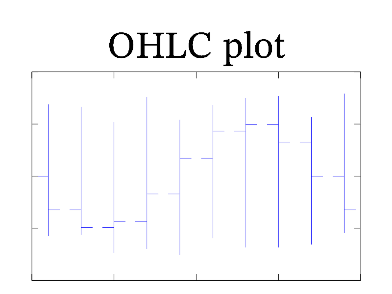
Next: param2 sample, Previous: ohlc sample, Up: All samples [Contents][Index]
Example of parametric plots for 1D data.
MGL code:
new x 100 'sin(pi*x)' new y 100 'cos(pi*x)' new z 100 'sin(2*pi*x)' new c 100 'cos(2*pi*x)' subplot 4 3 0:rotate 40 60:box:plot x y z subplot 4 3 1:rotate 40 60:box:area x y z subplot 4 3 2:rotate 40 60:box:tens x y z c subplot 4 3 3:rotate 40 60:box:bars x y z subplot 4 3 4:rotate 40 60:box:stem x y z subplot 4 3 5:rotate 40 60:box:textmark x y z c*2 '\alpha' subplot 4 3 6:rotate 40 60:box:tube x y z c/10 subplot 4 3 7:rotate 40 60:box:mark x y z c 's' subplot 4 3 8:box:error x y z/10 c/10 subplot 4 3 9:rotate 40 60:box:step x y z subplot 4 3 10:rotate 40 60:box:torus x z 'z';light on subplot 4 3 11:rotate 40 60:box:label x y z '%z'
C++ code:
void smgl_param1(mglGraph *gr) // 1d parametric plots
{
mglData x(100), y(100), z(100), c(100);
gr->Fill(x,"sin(pi*x)"); gr->Fill(y,"cos(pi*x)");
gr->Fill(z,"sin(2*pi*x)"); gr->Fill(c,"cos(2*pi*x)");
gr->SubPlot(4,3,0); gr->Rotate(40,60); gr->Box(); gr->Plot(x,y,z);
gr->SubPlot(4,3,1); gr->Rotate(40,60); gr->Box(); gr->Area(x,y,z);
gr->SubPlot(4,3,2); gr->Rotate(40,60); gr->Box(); gr->Tens(x,y,z,c);
gr->SubPlot(4,3,3); gr->Rotate(40,60); gr->Box(); gr->Bars(x,y,z);
gr->SubPlot(4,3,4); gr->Rotate(40,60); gr->Box(); gr->Stem(x,y,z);
gr->SubPlot(4,3,5); gr->Rotate(40,60); gr->Box(); gr->TextMark(x,y,z,c*2,"\\alpha");
gr->SubPlot(4,3,6); gr->Rotate(40,60); gr->Box(); gr->Tube(x,y,z,c/10,"","light on");
gr->SubPlot(4,3,7); gr->Rotate(40,60); gr->Box(); gr->Mark(x,y,z,c,"s");
gr->SubPlot(4,3,8); gr->Rotate(40,60); gr->Box(); gr->Error(x,y,z/10,c/10);
gr->SubPlot(4,3,9); gr->Rotate(40,60); gr->Box(); gr->Step(x,y,z);
gr->SubPlot(4,3,10);gr->Rotate(40,60); gr->Box(); gr->Torus(x,z,"z","light on");
gr->SubPlot(4,3,11);gr->Rotate(40,60); gr->Box(); gr->Label(x,y,z,"%z");
}
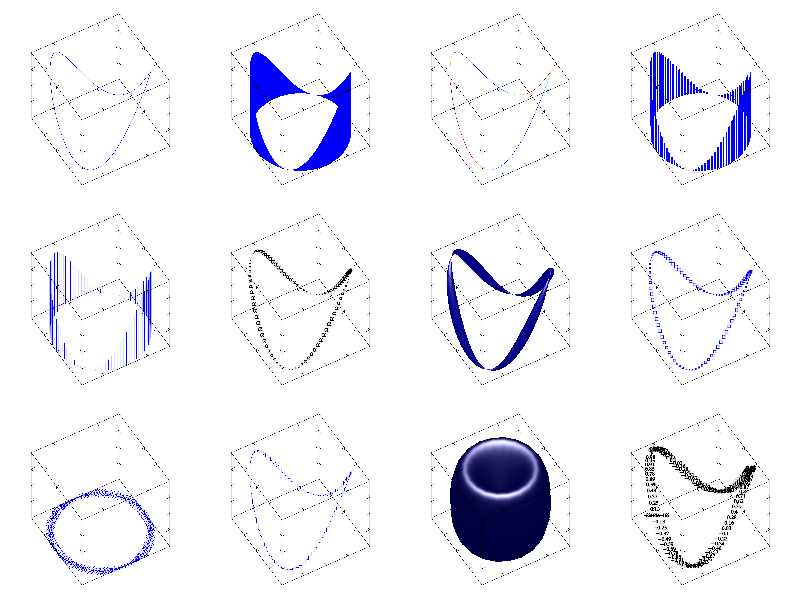
Next: param3 sample, Previous: param1 sample, Up: All samples [Contents][Index]
Example of parametric plots for 2D data.
MGL code:
new x 100 100 'sin(pi*(x+y)/2)*cos(pi*y/2)' new y 100 100 'cos(pi*(x+y)/2)*cos(pi*y/2)' new z 100 100 'sin(pi*y/2)' new c 100 100 'cos(pi*x)' subplot 4 4 0:rotate 40 60:box:surf x y z subplot 4 4 1:rotate 40 60:box:surfc x y z c subplot 4 4 2:rotate 40 60:box:surfa x y z c;alpha 1 subplot 4 4 3:rotate 40 60:box:mesh x y z;meshnum 10 subplot 4 4 4:rotate 40 60:box:tile x y z;meshnum 10 subplot 4 4 5:rotate 40 60:box:tiles x y z c;meshnum 10 subplot 4 4 6:rotate 40 60:box:axial x y z;alpha 0.5;light on subplot 4 4 7:rotate 40 60:box:cont x y z subplot 4 4 8:rotate 40 60:box:contf x y z;light on:contv x y z;light on subplot 4 4 9:rotate 40 60:box:belt x y z 'x';meshnum 10;light on subplot 4 4 10:rotate 40 60:box:dens x y z;alpha 0.5 subplot 4 4 11:rotate 40 60:box fall x y z 'g';meshnum 10:fall x y z 'rx';meshnum 10 subplot 4 4 12:rotate 40 60:box:belt x y z '';meshnum 10;light on subplot 4 4 13:rotate 40 60:box:boxs x y z '';meshnum 10;light on subplot 4 4 14:rotate 40 60:box:boxs x y z '#';meshnum 10;light on subplot 4 4 15:rotate 40 60:box:boxs x y z '@';meshnum 10;light on
C++ code:
void smgl_param2(mglGraph *gr) // 2d parametric plots
{
mglData x(100,100), y(100,100), z(100,100), c(100,100);
gr->Fill(x,"sin(pi*(x+y)/2)*cos(pi*y/2)"); gr->Fill(y,"cos(pi*(x+y)/2)*cos(pi*y/2)");
gr->Fill(z,"sin(pi*y/2)"); gr->Fill(c,"cos(pi*x)");
gr->SubPlot(4,4,0); gr->Rotate(40,60); gr->Box(); gr->Surf(x,y,z);
gr->SubPlot(4,4,1); gr->Rotate(40,60); gr->Box(); gr->SurfC(x,y,z,c);
gr->SubPlot(4,4,2); gr->Rotate(40,60); gr->Box(); gr->SurfA(x,y,z,c,"","alpha 1");
gr->SubPlot(4,4,3); gr->Rotate(40,60); gr->Box(); gr->Mesh(x,y,z,"","meshnum 10");
gr->SubPlot(4,4,4); gr->Rotate(40,60); gr->Box(); gr->Tile(x,y,z,"","meshnum 10");
gr->SubPlot(4,4,5); gr->Rotate(40,60); gr->Box(); gr->TileS(x,y,z,c,"","meshnum 10");
gr->SubPlot(4,4,6); gr->Rotate(40,60); gr->Box(); gr->Axial(x,y,z,"","alpha 0.5;light on");
gr->SubPlot(4,4,7); gr->Rotate(40,60); gr->Box(); gr->Cont(x,y,z);
gr->SubPlot(4,4,8); gr->Rotate(40,60); gr->Box(); gr->ContF(x,y,z,"","light on"); gr->ContV(x,y,z,"","light on");
gr->SubPlot(4,4,9); gr->Rotate(40,60); gr->Box(); gr->Belt(x,y,z,"x","meshnum 10;light on");
gr->SubPlot(4,4,10);gr->Rotate(40,60); gr->Box(); gr->Dens(x,y,z,"","alpha 0.5");
gr->SubPlot(4,4,11);gr->Rotate(40,60); gr->Box();
gr->Fall(x,y,z,"g","meshnum 10"); gr->Fall(x,y,z,"rx","meshnum 10");
gr->SubPlot(4,4,12); gr->Rotate(40,60); gr->Box(); gr->Belt(x,y,z,"","meshnum 10;light on");
gr->SubPlot(4,4,13); gr->Rotate(40,60); gr->Box(); gr->Boxs(x,y,z,"","meshnum 10;light on");
gr->SubPlot(4,4,14); gr->Rotate(40,60); gr->Box(); gr->Boxs(x,y,z,"#","meshnum 10");
gr->SubPlot(4,4,15); gr->Rotate(40,60); gr->Box(); gr->Boxs(x,y,z,"@","meshnum 10;light on");
}
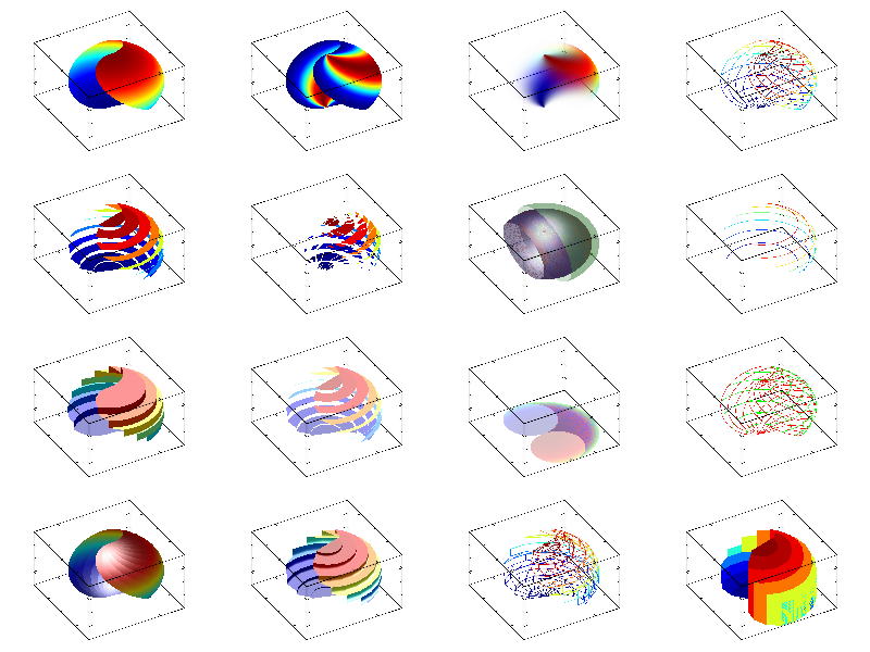
Next: paramv sample, Previous: param2 sample, Up: All samples [Contents][Index]
Example of parametric plots for 3D data.
MGL code:
new x 50 50 50 '(x+2)/3*sin(pi*y/2)' new y 50 50 50 '(x+2)/3*cos(pi*y/2)' new z 50 50 50 'z' new c 50 50 50 '-2*(x^2+y^2+z^4-z^2)+0.2' new d 50 50 50 '1-2*tanh(2*(x+y)^2)' alpha on:light on subplot 4 3 0:rotate 40 60:box:surf3 x y z c subplot 4 3 1:rotate 40 60:box:surf3c x y z c d subplot 4 3 2:rotate 40 60:box:surf3a x y z c d subplot 4 3 3:rotate 40 60:box:cloud x y z c subplot 4 3 4:rotate 40 60:box:cont3 x y z c:cont3 x y z c 'x':cont3 x y z c 'z' subplot 4 3 5:rotate 40 60:box:contf3 x y z c:contf3 x y z c 'x':contf3 x y z c 'z' subplot 4 3 6:rotate 40 60:box:dens3 x y z c:dens3 x y z c 'x':dens3 x y z c 'z' subplot 4 3 7:rotate 40 60:box:dots x y z c;meshnum 15 subplot 4 3 8:rotate 40 60:box:densx c '' 0:densy c '' 0:densz c '' 0 subplot 4 3 9:rotate 40 60:box:contx c '' 0:conty c '' 0:contz c '' 0 subplot 4 3 10:rotate 40 60:box:contfx c '' 0:contfy c '' 0:contfz c '' 0
C++ code:
void smgl_param3(mglGraph *gr) // 3d parametric plots
{
mglData x(50,50,50), y(50,50,50), z(50,50,50), c(50,50,50), d(50,50,50);
gr->Fill(x,"(x+2)/3*sin(pi*y/2)"); gr->Fill(y,"(x+2)/3*cos(pi*y/2)"); gr->Fill(z,"z");
gr->Fill(c,"-2*(x^2+y^2+z^4-z^2)+0.2"); gr->Fill(d,"1-2*tanh(2*(x+y)^2)");
gr->Light(true); gr->Alpha(true);
gr->SubPlot(4,3,0); gr->Rotate(40,60); gr->Box(); gr->Surf3(x,y,z,c);
gr->SubPlot(4,3,1); gr->Rotate(40,60); gr->Box(); gr->Surf3C(x,y,z,c,d);
gr->SubPlot(4,3,2); gr->Rotate(40,60); gr->Box(); gr->Surf3A(x,y,z,c,d);
gr->SubPlot(4,3,3); gr->Rotate(40,60); gr->Box(); gr->Cloud(x,y,z,c);
gr->SubPlot(4,3,4); gr->Rotate(40,60); gr->Box(); gr->Cont3(x,y,z,c); gr->Cont3(x,y,z,c,"x"); gr->Cont3(x,y,z,c,"z");
gr->SubPlot(4,3,5); gr->Rotate(40,60); gr->Box(); gr->ContF3(x,y,z,c);gr->ContF3(x,y,z,c,"x");gr->ContF3(x,y,z,c,"z");
gr->SubPlot(4,3,6); gr->Rotate(40,60); gr->Box(); gr->Dens3(x,y,z,c); gr->Dens3(x,y,z,c,"x"); gr->Dens3(x,y,z,c,"z");
gr->SubPlot(4,3,7); gr->Rotate(40,60); gr->Box(); gr->Dots(x,y,z,c,"","meshnum 15");
gr->SubPlot(4,3,8); gr->Rotate(40,60); gr->Box(); gr->DensX(c,"",0); gr->DensY(c,"",0); gr->DensZ(c,"",0);
gr->SubPlot(4,3,9); gr->Rotate(40,60); gr->Box(); gr->ContX(c,"",0); gr->ContY(c,"",0); gr->ContZ(c,"",0);
gr->SubPlot(4,3,10);gr->Rotate(40,60); gr->Box(); gr->ContFX(c,"",0); gr->ContFY(c,"",0); gr->ContFZ(c,"",0);
}
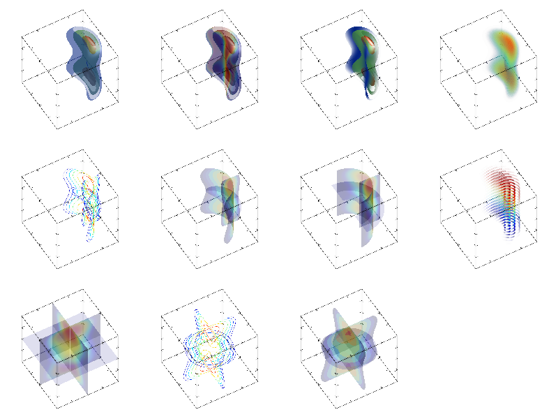
Next: parser sample, Previous: param3 sample, Up: All samples [Contents][Index]
Example of parametric plots for vector fields.
MGL code:
new x 20 20 20 '(x+2)/3*sin(pi*y/2)'
new y 20 20 20 '(x+2)/3*cos(pi*y/2)'
new z 20 20 20 'z+x'
new ex 20 20 20 'x'
new ey 20 20 20 'x^2+y'
new ez 20 20 20 'y^2+z'
new x1 50 50 '(x+2)/3*sin(pi*y/2)'
new y1 50 50 '(x+2)/3*cos(pi*y/2)'
new e1 50 50 'x'
new e2 50 50 'x^2+y'
subplot 3 3 0:rotate 40 60:box:vect x1 y1 e1 e2
subplot 3 3 1:rotate 40 60:box:flow x1 y1 e1 e2
subplot 3 3 2:rotate 40 60:box:pipe x1 y1 e1 e2
subplot 3 3 3:rotate 40 60:box:dew x1 y1 e1 e2
subplot 3 3 4:rotate 40 60:box:vect x y z ex ey ez
subplot 3 3 5:rotate 40 60:box
vect3 x y z ex ey ez:vect3 x y z ex ey ez 'x':vect3 x y z ex ey ez 'z'
grid3 x y z z '{r9}':grid3 x y z z '{g9}x':grid3 x y z z '{b9}z'
subplot 3 3 6:rotate 40 60:box:flow x y z ex ey ez
subplot 3 3 7:rotate 40 60:box:pipe x y z ex ey ez
C++ code:
void smgl_paramv(mglGraph *gr) // parametric plots for vector field
{
mglData x(20,20,20), y(20,20,20), z(20,20,20), ex(20,20,20), ey(20,20,20), ez(20,20,20);
gr->Fill(x,"(x+2)/3*sin(pi*y/2)"); gr->Fill(y,"(x+2)/3*cos(pi*y/2)"); gr->Fill(z,"x+z");
gr->Fill(ex,"x"); gr->Fill(ey,"x^2+y"); gr->Fill(ez,"y^2+z");
mglData x1(20,20), y1(20,20), e1(20,20), e2(20,20);
gr->Fill(x1,"(x+2)/3*sin(pi*y/2)"); gr->Fill(y1,"(x+2)/3*cos(pi*y/2)");
gr->Fill(e1,"x"); gr->Fill(e2,"x^2+y");
gr->SubPlot(3,3,0); gr->Rotate(40,60); gr->Box(); gr->Vect(x1,y1,e1,e2);
gr->SubPlot(3,3,1); gr->Rotate(40,60); gr->Box(); gr->Flow(x1,y1,e1,e2);
gr->SubPlot(3,3,2); gr->Rotate(40,60); gr->Box(); gr->Pipe(x1,y1,e1,e2);
gr->SubPlot(3,3,3); gr->Rotate(40,60); gr->Box(); gr->Dew(x1,y1,e1,e2);
gr->SubPlot(3,3,4); gr->Rotate(40,60); gr->Box(); gr->Vect(x,y,z,ex,ey,ez);
gr->SubPlot(3,3,5); gr->Rotate(40,60); gr->Box();
gr->Vect3(x,y,z,ex,ey,ez); gr->Vect3(x,y,z,ex,ey,ez,"x"); gr->Vect3(x,y,z,ex,ey,ez,"z");
gr->Grid3(x,y,z,z,"{r9}"); gr->Grid3(x,y,z,z,"{g9}x"); gr->Grid3(x,y,z,z,"{b9}z");
gr->SubPlot(3,3,6); gr->Rotate(40,60); gr->Box(); gr->Flow(x,y,z,ex,ey,ez);
gr->SubPlot(3,3,7); gr->Rotate(40,60); gr->Box(); gr->Pipe(x,y,z,ex,ey,ez);
}
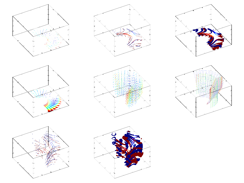
Next: pde sample, Previous: paramv sample, Up: All samples [Contents][Index]
Basic MGL script.
MGL code:
title 'MGL parser sample' # call function call 'sample' # ordinary for-loop for $0 -1 1 0.1 if $0<0:line 0 0 1 $0 'r':else:line 0 0 1 $0 'g':endif next # if-elseif-else for $i -1 1 0.5 if $i<0 text 1.1 $i '$i' 'b' elseif $i>0 text 1.1 $i '$i' 'r' else text 1.1 $i '$i' endif next # ordinary do-while do defnum $i $i-0.2 line 0 0 $i 1 'b' while $i>0 # do-next-break do defnum $i $i-0.2 if $i<-1 then break line 0 0 $i 1 'm' next # for-while-continue for $i -5 10 text $i/5 1.1 'a'+($i+5) if $i<0 text $i/5-0.06 1.1 '--' 'b' elseif mod($i,2)=0 text $i/5-0.06 1.1 '~' 'r' else # NOTE: 'continue' bypass the 'while'! continue endif # NOTE: 'while' limit the actual number of iterations while $i<5 # nested loops for $i 0 1 0.1 for $j 0 1 0.1 ball $i $j if $j>0.5 then continue ball $i $j 'b+' next next func 'sample' new dat 100 'sin(2*pi*(i/99+1))' plot dat;xrange -1 0 box:axis xlabel 'x':ylabel 'y' return
C++ code:
void smgl_parser(mglGraph *gr) // example of MGL parsing
{ // NOTE: MGL version show much more variants of loops and conditions.
gr->Title("MGL parser sample");
double a[100]; // let a_i = sin(4*pi*x), x=0...1
for(int i=0;i<100;i++)a[i]=sin(2*M_PI*i/99);
mglParse *parser = new mglParse;
// Add MGL variable and set yours data to it.
mglData *d = dynamic_cast<mglData*>(parser->AddVar("dat"));
if(d) d->Set(a,100);
parser->Execute(gr, "plot dat; xrange -1 0\nbox\naxis");
// You may break script at any line do something
// and continue after that.
parser->Execute(gr, "xlabel 'x'\nylabel 'y'\nbox");
// Also you may use cycles or conditions in script.
parser->Execute(gr, "for $0 -1 1 0.1\nif $0<0\n"
"line 0 0 1 $0 'r':else:line 0 0 1 $0 'g'\n"
"endif\nnext");
// You may use for or do-while loops as C/C++ one
double i=1;
do {
char buf[64]; sprintf(buf,"line 0 0 %g 1 'b'",i);
parser->Execute(gr, buf); i=i-0.2;
} while(i>0);
// or as MGL one.
parser->Execute(gr, "for $i -1 1 0.5\n"
"if $i<0\ntext 1.1 $i '$i' 'b'\n"
"elseif $i>0\ntext 1.1 $i '$i' 'r'\n"
"else\ntext 1.1 $i '$i'\nendif\nnext\n");
// There are 'break' and 'continue' commands in MGL too.
// NOTE: 'next' act as "while(1)" in do-while loops.
parser->Execute(gr, "do\ndefnum $i $i-0.2\n"
"if $i<-1 then break\nline 0 0 $i 1 'm'\nnext\n");
// One issue with 'continue' -- it bypass 'while' checking
parser->Execute(gr, "for $i -5 10\ntext $i/5 1.1 'a'+($i+5)\nif $i<0\n"
"text $i/5-0.06 1.1 '--' 'b'\n"
"elseif mod($i,2)=0\ntext $i/5-0.06 1.1 '~' 'r'\n"
"else\ncontinue\nendif\n"
// NOTE: 'while' limit the actual number of iterations in for-loop.
"while $i<5\n");
// Finally, MGL support nested loops too.
parser->Execute(gr, "for $i 0 1 0.1\nfor $j 0 1 0.1\nball $i $j\n"
"if $j>0.5 then continue\nball $i $j 'b+'\nnext\nnext\n");
// Clean up memory.
delete parser;
}
Next: pendelta sample, Previous: parser sample, Up: All samples [Contents][Index]
Example of pde solver.
MGL code:
new re 128 'exp(-48*(x+0.7)^2)':new im 128
pde a 'p^2+q^2-x-1+i*0.5*(z+x)*(z>-x)' re im 0.01 30
transpose a
subplot 1 1 0 '<_':title 'PDE solver'
axis:xlabel '\i x':ylabel '\i z'
crange 0 1:dens a 'wyrRk'
fplot '-x' 'k|'
text 0 0.95 'Equation: ik_0\partial_zu + \Delta u + x\cdot u + i \frac{x+z}{2}\cdot u = 0\n{}absorption: (x+z)/2 for x+z>0'
C++ code:
void smgl_pde(mglGraph *gr) // PDE sample
{
mglData a,re(128),im(128);
gr->Fill(re,"exp(-48*(x+0.7)^2)");
a = gr->PDE("p^2+q^2-x-1+i*0.5*(z+x)*(z>-x)", re, im, 0.01, 30);
a.Transpose("yxz");
if(big!=3) {gr->SubPlot(1,1,0,"<_"); gr->Title("PDE solver"); }
gr->SetRange('c',0,1); gr->Dens(a,"wyrRk");
gr->Axis(); gr->Label('x', "\\i x"); gr->Label('y', "\\i z");
gr->FPlot("-x", "k|");
gr->Puts(mglPoint(0, 0.95), "Equation: ik_0\\partial_zu + \\Delta u + x\\cdot u + i \\frac{x+z}{2}\\cdot u = 0\nabsorption: (x+z)/2 for x+z>0");
}
Next: pipe sample, Previous: pde sample, Up: All samples [Contents][Index]
Example of pendelta for lines and glyphs smoothing.
MGL code:
quality 6 list a 0.25 0.5 1 2 4 for $0 0 4 pendelta a($0) define $1 0.5*$0-1 line -1 $1 1 $1 'r' text 0 $1 'delta=',a($0) next
C++ code:
void smgl_pendelta(mglGraph *gr)
{
double a[5]={0.25,0.5,1,2,4};
gr->SetQuality(6);
char buf[64];
for(int i=0;i<5;i++)
{
gr->SetPenDelta(a[i]);
gr->Line(mglPoint(-1,0.5*i-1), mglPoint(1,0.5*i-1),"r");
sprintf(buf,"delta=%g",a[i]);
gr->Puts(mglPoint(0,0.5*i-1),buf);
}
}
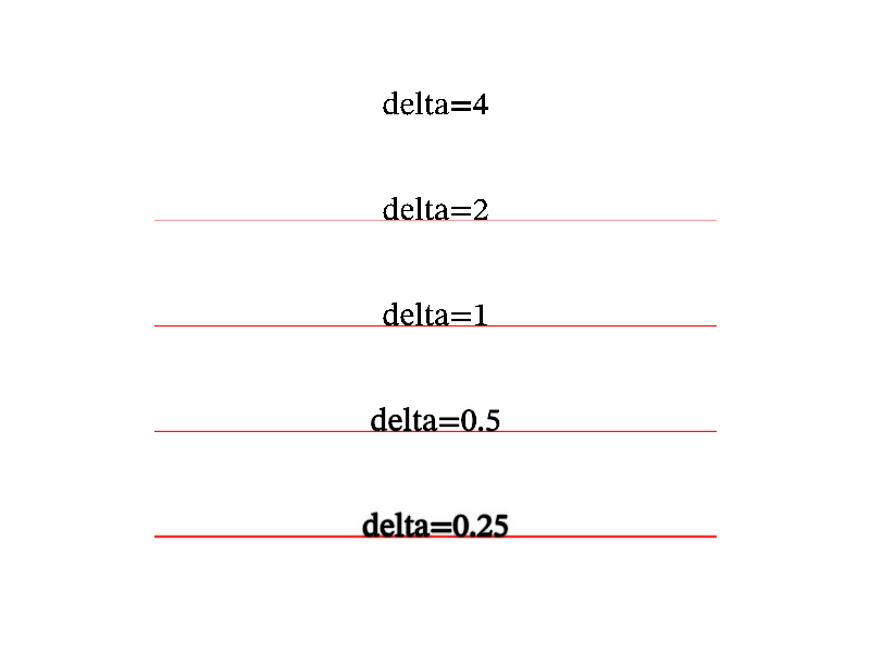
Next: plot sample, Previous: pendelta sample, Up: All samples [Contents][Index]
Function pipe is similar to flow but draw pipes (tubes) which radius is proportional to the amplitude of vector field. The color scheme is used for coloring (see Color scheme). At this warm color corresponds to normal flow (like attractor), cold one corresponds to inverse flow (like source).
MGL code:
call 'prepare2v' call 'prepare3v' subplot 2 2 0 '':title 'Pipe plot (default)':light on:box:pipe a b subplot 2 2 1 '':title '"i" style':box:pipe a b 'i' subplot 2 2 2 '':title 'from edges only':box:pipe a b '#' subplot 2 2 3:title '3d variant':rotate 50 60:box:pipe ex ey ez '' 0.1
C++ code:
void smgl_pipe(mglGraph *gr)
{
mglData a,b; mgls_prepare2v(&a,&b);
if(big!=3) {gr->SubPlot(2,2,0,""); gr->Title("Pipe plot (default)");}
gr->Light(true); gr->Box(); gr->Pipe(a,b);
if(big==3) return;
gr->SubPlot(2,2,1,""); gr->Title("'i' style"); gr->Box(); gr->Pipe(a,b,"i");
gr->SubPlot(2,2,2,""); gr->Title("'\\#' style"); gr->Box(); gr->Pipe(a,b,"#");
mglData ex,ey,ez; mgls_prepare3v(&ex,&ey,&ez);
gr->SubPlot(2,2,3); gr->Title("3d variant"); gr->Rotate(50,60);
gr->Box(); gr->Pipe(ex,ey,ez,"",0.1);
}

Next: pmap sample, Previous: pipe sample, Up: All samples [Contents][Index]
Function plot is most standard way to visualize 1D data array. By default, Plot use colors from palette. However, you can specify manual color/palette, and even set to use new color for each points by using ‘!’ style. Another feature is ‘ ’ style which draw only markers without line between points.
MGL code:
call 'prepare1d' subplot 2 2 0 '':title 'Plot plot (default)':box:plot y subplot 2 2 2 '':title ''!' style; 'rgb' palette':box:plot y 'o!rgb' subplot 2 2 3 '':title 'just markers':box:plot y ' +' new yc 30 'sin(pi*x)':new xc 30 'cos(pi*x)':new z 30 'x' subplot 2 2 1:title '3d variant':rotate 50 60:box:plot xc yc z 'rs'
C++ code:
void smgl_plot(mglGraph *gr)
{
mglData y; mgls_prepare1d(&y); gr->SetOrigin(0,0,0);
if(big!=3) { gr->SubPlot(2,2,0,""); gr->Title("Plot plot (default)"); }
gr->Box(); gr->Plot(y);
if(big==3) return;
gr->SubPlot(2,2,2,""); gr->Title("'!' style; 'rgb' palette"); gr->Box(); gr->Plot(y,"o!rgb");
gr->SubPlot(2,2,3,""); gr->Title("just markers"); gr->Box(); gr->Plot(y," +");
gr->SubPlot(2,2,1); gr->Title("3d variant"); gr->Rotate(50,60); gr->Box();
mglData yc(30), xc(30), z(30); z.Modify("2*x-1");
yc.Modify("sin(pi*(2*x-1))"); xc.Modify("cos(pi*2*x-pi)");
gr->Plot(xc,yc,z,"rs");
}

Next: primitives sample, Previous: plot sample, Up: All samples [Contents][Index]
Function pmap draw Poincare map – show intersections of the curve and the surface.
MGL code:
subplot 1 1 0 '<_^':title 'Poincare map sample' ode r 'cos(y)+sin(z);cos(z)+sin(x);cos(x)+sin(y)' 'xyz' [0.1,0,0] 0.1 100 rotate 40 60:copy x r(0):copy y r(1):copy z r(2) ranges x y z axis:plot x y z 'b' xlabel '\i x' 0:ylabel '\i y' 0:zlabel '\i z' pmap x y z z 'b#o' fsurf '0'
C++ code:
void smgl_pmap(mglGraph *gr)
{
gr->SubPlot(1,1,0,"<_^");
if(big!=3) gr->Title("Poincare map sample");
mglData ini(3); ini[0]=0.1;
mglData r(mglODE("cos(y)+sin(z);cos(z)+sin(x);cos(x)+sin(y)","xyz",ini,0.1,100));
mglData x(r.SubData(0)),y(r.SubData(1)), z(r.SubData(2));
gr->Rotate(40,60); gr->SetRanges(x,y,z);
gr->Axis(); gr->FSurf("0"); gr->Plot(x,y,z,"b");
gr->Label('x',"\\i x",0); gr->Label('y',"\\i y",0); gr->Label('z',"\\i z",0);
gr->Pmap(x,y,z,z, "b#o");
}
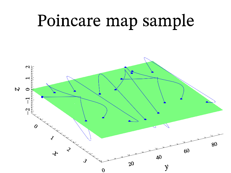
Next: projection sample, Previous: pmap sample, Up: All samples [Contents][Index]
Example of primitives: line, curve, rhomb, ellipse, face, sphere, drop, cone.
MGL code:
subplot 2 2 0 '':title 'Line, Curve, Rhomb, Ellipse' '' -1.5
line -1 -1 -0.5 1 'qAI'
curve -0.6 -1 1 1 0 1 1 1 'rA'
ball 0 -0.5 '*':ball 1 -0.1 '*'
rhomb 0 0.4 1 0.9 0.2 'b#'
rhomb 0 0 1 0.4 0.2 'cg@'
ellipse 0 -0.5 1 -0.1 0.2 'u#'
ellipse 0 -1 1 -0.6 0.2 'm@'
subplot 2 3 1 '':title 'Arc, Polygon, Symbol';size -1.2
arc -0.6 0 -0.6 0.3 180 '2kA':ball -0.6 0
polygon 0 0 0 0.4 6 'r'
new x 50 'cos(3*pi*x)':new y 50 'sin(pi*x)'
addsymbol 'a' x y
symbol 0.7 0 'a'
light on
subplot 2 3 3 '<^>' 0 -0.2:title 'Face[xyz]';size -1.5:rotate 50 60:box
facex 1 0 -1 1 1 'r':facey -1 -1 -1 1 1 'g':facez 1 -1 -1 -1 1 'b'
face -1 -1 1 -1 1 1 1 -1 0 1 1 1 'bmgr'
subplot 2 3 5 '':title 'Cone';size -1.5
cone -0.7 -0.3 0 -0.7 0.7 0.5 0.2 0.1 'b':text -0.7 -0.7 'no edges\n(default)';size -1.5
cone 0 -0.3 0 0 0.7 0.5 0.2 0.1 'g@':text 0 -0.7 'with edges\n("\@" style)';size -1.5
cone 0.7 -0.3 0 0.7 0.7 0.5 0.2 0 'Ggb':text 0.7 -0.7 '"arrow" with\n{}gradient';size -1.5
subplot 2 2 2 '':title 'Sphere and Drop'
line -0.9 0 1 0.9 0 1
text -0.9 0.4 'sh=0':drop -0.9 0 0 1 0.5 'r' 0:ball -0.9 0 1 'k'
text -0.3 0.6 'sh=0.33':drop -0.3 0 0 1 0.5 'r' 0.33:ball -0.3 0 1 'k'
text 0.3 0.8 'sh=0.67':drop 0.3 0 0 1 0.5 'r' 0.67:ball 0.3 0 1 'k'
text 0.9 1. 'sh=1':drop 0.9 0 0 1 0.5 'r' 1:ball 0.9 0 1 'k'
text -0.9 -1.1 'asp=0.33':drop -0.9 -0.7 0 1 0.5 'b' 0 0.33
text -0.3 -1.1 'asp=0.67':drop -0.3 -0.7 0 1 0.5 'b' 0 0.67
text 0.3 -1.1 'asp=1':drop 0.3 -0.7 0 1 0.5 'b' 0 1
text 0.9 -1.1 'asp=1.5':drop 0.9 -0.7 0 1 0.5 'b' 0 1.5
C++ code:
void smgl_primitives(mglGraph *gr) // flag #
{
gr->SubPlot(2,2,0,""); gr->Title("Line, Curve, Rhomb, Ellipse","",-1.5);
gr->Line(mglPoint(-1,-1),mglPoint(-0.5,1),"qAI");
gr->Curve(mglPoint(-0.6,-1),mglPoint(1,1),mglPoint(0,1),mglPoint(1,1),"rA");
gr->Rhomb(mglPoint(0,0.4),mglPoint(1,0.9),0.2,"b#");
gr->Rhomb(mglPoint(0,0),mglPoint(1,0.4),0.2,"cg@");
gr->Ellipse(mglPoint(0,-0.5),mglPoint(1,-0.1),0.2,"u#");
gr->Ellipse(mglPoint(0,-1),mglPoint(1,-0.6),0.2,"m@");
gr->Mark(mglPoint(0,-0.5),"*"); gr->Mark(mglPoint(1,-0.1),"*");
gr->SubPlot(2,3,1,""); gr->Title("Arc, Polygon, Symbol","", -1.2*2);
gr->Arc(mglPoint(-0.6,0), mglPoint(-0.6,0.3), 180, "2kA"); gr->Ball(-0.6,0);
gr->Polygon(mglPoint(), mglPoint(0,0.4), 6, "r");
mglData x(50), y(50); gr->Fill(x,"cos(3*pi*x)"); gr->Fill(y,"sin(pi*x)");
gr->DefineSymbol('a',x,y); gr->Symbol(mglPoint(0.7),'a');
gr->Light(true);
gr->SubPlot(2,3,3,"<^>",0,-0.2); gr->Title("Face[xyz]", "", -1.5*2);
gr->Rotate(50,60); gr->Box();
gr->FaceX(mglPoint(1,0,-1),1,1,"r");
gr->FaceY(mglPoint(-1,-1,-1),1,1,"g");
gr->FaceZ(mglPoint(1,-1,-1),-1,1,"b");
gr->Face(mglPoint(-1,-1,1),mglPoint(-1,1,1),mglPoint(1,-1,0),mglPoint(1,1,1),"bmgr");
gr->SubPlot(2,3,5,""); gr->Title("Cone", "", -1.5*2);
gr->Cone(mglPoint(-0.7,-0.3),mglPoint(-0.7,0.7,0.5),0.2,0.1,"b");
gr->Puts(mglPoint(-0.7,-0.7),"no edges\n(default)","", -1.5);
gr->Cone(mglPoint(0,-0.3),mglPoint(0,0.7,0.5),0.2,0.1,"g@");
gr->Puts(mglPoint(0,-0.7),"with edges\n('\\@' style)","", -1.5);
gr->Cone(mglPoint(0.7,-0.3),mglPoint(0.7,0.7,0.5),0.2,0,"ry");
gr->Puts(mglPoint(0.7,-0.7),"'arrow' with\ngradient","", -1.5);
gr->SubPlot(2,2,2,""); gr->Title("Sphere and Drop"); gr->Alpha(false);
gr->Puts(mglPoint(-0.9,0.4),"sh=0"); gr->Ball(mglPoint(-0.9,0,1),'k');
gr->Drop(mglPoint(-0.9,0),mglPoint(0,1),0.5,"r",0);
gr->Puts(mglPoint(-0.3,0.6),"sh=0.33"); gr->Ball(mglPoint(-0.3,0,1),'k');
gr->Drop(mglPoint(-0.3,0),mglPoint(0,1),0.5,"r",0.33);
gr->Puts(mglPoint(0.3,0.8),"sh=0.67"); gr->Ball(mglPoint(0.3,0,1),'k');
gr->Drop(mglPoint(0.3,0),mglPoint(0,1),0.5,"r",0.67);
gr->Puts(mglPoint(0.9,1),"sh=1"); gr->Ball(mglPoint(0.9,0,1),'k');
gr->Drop(mglPoint(0.9,0),mglPoint(0,1),0.5,"r",1);
gr->Line(mglPoint(-0.9,0,1),mglPoint(0.9,0,1),"b");
gr->Puts(mglPoint(-0.9,-1.1),"asp=0.33");
gr->Drop(mglPoint(-0.9,-0.7),mglPoint(0,1),0.5,"b",0,0.33);
gr->Puts(mglPoint(-0.3,-1.1),"asp=0.67");
gr->Drop(mglPoint(-0.3,-0.7),mglPoint(0,1),0.5,"b",0,0.67);
gr->Puts(mglPoint(0.3,-1.1),"asp=1");
gr->Drop(mglPoint(0.3,-0.7),mglPoint(0,1),0.5,"b",0,1);
gr->Puts(mglPoint(0.9,-1.1),"asp=1.5");
gr->Drop(mglPoint(0.9,-0.7),mglPoint(0,1),0.5,"b",0,1.5);
}
Next: projection5 sample, Previous: primitives sample, Up: All samples [Contents][Index]
Example of plot projection (ternary=4).
MGL code:
ranges 0 1 0 1 0 1 new x 50 '0.25*(1+cos(2*pi*x))' new y 50 '0.25*(1+sin(2*pi*x))' new z 50 'x' new a 20 30 '30*x*y*(1-x-y)^2*(x+y<1)' new rx 10 'rnd':new ry 10:fill ry '(1-v)*rnd' rx light on title 'Projection sample':ternary 4:rotate 50 60 box:axis:grid plot x y z 'r2':surf a '#' xlabel 'X':ylabel 'Y':zlabel 'Z'
C++ code:
void smgl_projection(mglGraph *gr) // flag #
{
gr->SetRanges(0,1,0,1,0,1);
mglData x(50),y(50),z(50),rx(10),ry(10), a(20,30);
a.Modify("30*x*y*(1-x-y)^2*(x+y<1)");
x.Modify("0.25*(1+cos(2*pi*x))");
y.Modify("0.25*(1+sin(2*pi*x))");
rx.Modify("rnd"); ry.Modify("(1-v)*rnd",rx);
z.Modify("x");
if(big!=3) gr->Title("Projection sample");
gr->Ternary(4);
gr->Rotate(50,60); gr->Light(true);
gr->Plot(x,y,z,"r2"); gr->Surf(a,"#");
gr->Axis(); gr->Grid(); gr->Box();
gr->Label('x',"X",1); gr->Label('y',"Y",1); gr->Label('z',"Z",1);
}
Next: pulse sample, Previous: projection sample, Up: All samples [Contents][Index]
Example of plot projection in ternary coordinates (ternary=5).
MGL code:
ranges 0 1 0 1 0 1 new x 50 '0.25*(1+cos(2*pi*x))' new y 50 '0.25*(1+sin(2*pi*x))' new z 50 'x' new a 20 30 '30*x*y*(1-x-y)^2*(x+y<1)' new rx 10 'rnd':new ry 10:fill ry '(1-v)*rnd' rx light on title 'Projection sample (ternary)':ternary 5:rotate 50 60 box:axis:grid plot x y z 'r2':surf a '#' xlabel 'X':ylabel 'Y':zlabel 'Z'
C++ code:
void smgl_projection5(mglGraph *gr) // flag #
{
gr->SetRanges(0,1,0,1,0,1);
mglData x(50),y(50),z(50),rx(10),ry(10), a(20,30);
a.Modify("30*x*y*(1-x-y)^2*(x+y<1)");
x.Modify("0.25*(1+cos(2*pi*x))");
y.Modify("0.25*(1+sin(2*pi*x))");
rx.Modify("rnd"); ry.Modify("(1-v)*rnd",rx);
z.Modify("x");
if(big!=3) gr->Title("Projection sample (ternary)");
gr->Ternary(5);
gr->Rotate(50,60); gr->Light(true);
gr->Plot(x,y,z,"r2"); gr->Surf(a,"#");
gr->Axis(); gr->Grid(); gr->Box();
gr->Label('x',"X",1); gr->Label('y',"Y",1); gr->Label('z',"Z",1);
}
Next: qo2d sample, Previous: projection5 sample, Up: All samples [Contents][Index]
Example of pulse parameter determining.
MGL code:
subplot 1 1 0 '<_':title 'Pulse sample' new a 100 'exp(-6*x^2)':ranges 0 a.nx-1 0 1 axis:plot a pulse b a 'x' define m a.max line b(1) 0 b(1) m 'r=' line b(1)-b(3)/2 0 b(1)-b(3)/2 m 'm|' line b(1)+b(3)/2 0 b(1)+b(3)/2 m 'm|' line 0 0.5*m a.nx-1 0.5*m 'h' new x 100 'x' plot b(0)*(1-((x-b(1))/b(2))^2) 'g'
C++ code:
void smgl_pulse(mglGraph *gr)
{
gr->SubPlot(1,1,0,"<_");
if(big!=3) gr->Title("Pulse sample");
mglData a(100); gr->Fill(a,"exp(-6*x^2)");
gr->SetRanges(0, a.nx-1, 0, 1);
gr->Axis(); gr->Plot(a);
mglData b(a.Pulse('x'));
double m = b[0];
gr->Line(mglPoint(b[1],0), mglPoint(b[1],m),"r=");
gr->Line(mglPoint(b[1]-b[3]/2,0), mglPoint(b[1]-b[3]/2,m),"m|");
gr->Line(mglPoint(b[1]+b[3]/2,0), mglPoint(b[1]+b[3]/2,m),"m|");
gr->Line(mglPoint(0,m/2), mglPoint(a.nx-1,m/2),"h");
char func[128]; sprintf(func,"%g*(1-((x-%g)/%g)^2)",b[0],b[1],b[2]);
gr->FPlot(func,"g");
}
Next: quality0 sample, Previous: pulse sample, Up: All samples [Contents][Index]
Example of PDE solving by quasioptical approach qo2d.
MGL code:
define $1 'p^2+q^2-x-1+i*0.5*(y+x)*(y>-x)' subplot 1 1 0 '<_':title 'Beam and ray tracing' ray r $1 -0.7 -1 0 0 0.5 0 0.02 2:plot r(0) r(1) 'k' axis:xlabel '\i x':ylabel '\i z' new re 128 'exp(-48*x^2)':new im 128 new xx 1:new yy 1 qo2d a $1 re im r 1 30 xx yy crange 0 1:dens xx yy a 'wyrRk':fplot '-x' 'k|' text 0 0.85 'absorption: (x+y)/2 for x+y>0' text 0.7 -0.05 'central ray'
C++ code:
void smgl_qo2d(mglGraph *gr)
{
mglData r, xx, yy, a, im(128), re(128);
const char *ham = "p^2+q^2-x-1+i*0.5*(y+x)*(y>-x)";
r = mglRay(ham, mglPoint(-0.7, -1), mglPoint(0, 0.5), 0.02, 2);
if(big!=3) {gr->SubPlot(1,1,0,"<_"); gr->Title("Beam and ray tracing");}
gr->Plot(r.SubData(0), r.SubData(1), "k");
gr->Axis(); gr->Label('x', "\\i x"); gr->Label('y', "\\i y");
// now start beam tracing
gr->Fill(re,"exp(-48*x^2)");
a = mglQO2d(ham, re, im, r, xx, yy, 1, 30);
gr->SetRange('c',0, 1);
gr->Dens(xx, yy, a, "wyrRk");
gr->FPlot("-x", "k|");
gr->Puts(mglPoint(0, 0.85), "absorption: (x+y)/2 for x+y>0");
gr->Puts(mglPoint(0.7, -0.05), "central ray");
}
Next: quality1 sample, Previous: qo2d sample, Up: All samples [Contents][Index]
Show all kind of primitives in quality=0.
MGL code:
quality 0
subplot 3 2 0:define y 0.95
define d 0.3:define x0 0.2:define x1 0.5:define x2 0.6
line x0 1-0*d x1 1-0*d 'k-':text x2 y-0*d 'Solid `-`' ':rL'
line x0 1-1*d x1 1-1*d 'k|':text x2 y-1*d 'Long Dash `|`' ':rL'
line x0 1-2*d x1 1-2*d 'k;':text x2 y-2*d 'Dash 1;`' ':rL'
line x0 1-3*d x1 1-3*d 'k=':text x2 y-3*d 'Small dash `=`' ':rL'
line x0 1-4*d x1 1-4*d 'kj':text x2 y-4*d 'Dash-dot `j`' ':rL'
line x0 1-5*d x1 1-5*d 'ki':text x2 y-5*d 'Small dash-dot `i`' ':rL'
line x0 1-6*d x1 1-6*d 'k:':text x2 y-6*d 'Dots `:`' ':rL'
line x0 1-7*d x1 1-7*d 'k ':text x2 y-7*d 'None ``' ':rL'
define d 0.25:define x0 -0.8:define x1 -1:define x2 -0.05
ball x1 5*d 'k.':text x0 5*d '.' ':rL'
ball x1 4*d 'k+':text x0 4*d '+' ':rL'
ball x1 3*d 'kx':text x0 3*d 'x' ':rL'
ball x1 2*d 'k*':text x0 2*d '*' ':rL'
ball x1 d 'ks':text x0 d 's' ':rL'
ball x1 0 'kd':text x0 0 'd' ':rL'
ball x1 -d 0 'ko':text x0 y-d 'o' ':rL'
ball x1 -2*d 0 'k^':text x0 -2*d '\^' ':rL'
ball x1 -3*d 0 'kv':text x0 -3*d 'v' ':rL'
ball x1 -4*d 0 'k<':text x0 -4*d '<' ':rL'
ball x1 -5*d 0 'k>':text x0 -5*d '>' ':rL'
define x0 -0.3:define x1 -0.5
ball x1 5*d 'k#.':text x0 5*d '\#.' ':rL'
ball x1 4*d 'k#+':text x0 4*d '\#+' ':rL'
ball x1 3*d 'k#x':text x0 3*d '\#x' ':rL'
ball x1 2*d 'k#*':text x0 2*d '\#*' ':rL'
ball x1 d 'k#s':text x0 d '\#s' ':rL'
ball x1 0 'k#d':text x0 0 '\#d' ':rL'
ball x1 -d 0 'k#o':text x0 -d '\#o' ':rL'
ball x1 -2*d 0 'k#^':text x0 -2*d '\#\^' ':rL'
ball x1 -3*d 0 'k#v':text x0 -3*d '\#v' ':rL'
ball x1 -4*d 0 'k#<':text x0 -4*d '\#<' ':rL'
ball x1 -5*d 0 'k#>':text x0 -5*d '\#>' ':rL'
subplot 3 2 1
define a 0.1:define b 0.4:define c 0.5
line a 1 b 1 'k-A':text c 1 'Style `A` or `A\_`' ':rL'
line a 0.8 b 0.8 'k-V':text c 0.8 'Style `V` or `V\_`' ':rL'
line a 0.6 b 0.6 'k-K':text c 0.6 'Style `K` or `K\_`' ':rL'
line a 0.4 b 0.4 'k-I':text c 0.4 'Style `I` or `I\_`' ':rL'
line a 0.2 b 0.2 'k-D':text c 0.2 'Style `D` or `D\_`' ':rL'
line a 0 b 0 'k-S':text c 0 'Style `S` or `S\_`' ':rL'
line a -0.2 b -0.2 'k-O':text c -0.2 'Style `O` or `O\_`' ':rL'
line a -0.4 b -0.4 'k-T':text c -0.4 'Style `T` or `T\_`' ':rL'
line a -0.6 b -0.6 'k-_':text c -0.6 'Style `\_` or none' ':rL'
line a -0.8 b -0.8 'k-AS':text c -0.8 'Style `AS`' ':rL'
line a -1 b -1 'k-_A':text c -1 'Style `\_A`' ':rL'
define a -1:define b -0.7:define c -0.6
line a 1 b 1 'kAA':text c 1 'Style `AA`' ':rL'
line a 0.8 b 0.8 'kVV':text c 0.8 'Style `VV`' ':rL'
line a 0.6 b 0.6 'kKK':text c 0.6 'Style `KK`' ':rL'
line a 0.4 b 0.4 'kII':text c 0.4 'Style `II`' ':rL'
line a 0.2 b 0.2 'kDD':text c 0.2 'Style `DD`' ':rL'
line a 0 b 0 'kSS':text c 0 'Style `SS`' ':rL'
line a -0.2 b -0.2 'kOO':text c -0.2 'Style `OO`' ':rL'
line a -0.4 b -0.4 'kTT':text c -0.4 'Style `TT`' ':rL'
line a -0.6 b -0.6 'k-__':text c -0.6 'Style `\_\_`' ':rL'
line a -0.8 b -0.8 'k-VA':text c -0.8 'Style `VA`' ':rL'
line a -1 b -1 'k-AV':text c -1 'Style `AV`' ':rL'
subplot 3 2 2
#LENUQ
facez -1 -1 0 0.4 0.3 'L#':text -0.8 -0.9 'L' 'w:C' -1.4
facez -0.6 -1 0 0.4 0.3 'E#':text -0.4 -0.9 'E' 'w:C' -1.4
facez -0.2 -1 0 0.4 0.3 'N#':text 0 -0.9 'N' 'w:C' -1.4
facez 0.2 -1 0 0.4 0.3 'U#':text 0.4 -0.9 'U' 'w:C' -1.4
facez 0.6 -1 0 0.4 0.3 'Q#':text 0.8 -0.9 'Q' 'w:C' -1.4
#lenuq
facez -1 -0.7 0 0.4 0.3 'l#':text -0.8 -0.6 'l' 'k:C' -1.4
facez -0.6 -0.7 0 0.4 0.3 'e#':text -0.4 -0.6 'e' 'k:C' -1.4
facez -0.2 -0.7 0 0.4 0.3 'n#':text 0 -0.6 'n' 'k:C' -1.4
facez 0.2 -0.7 0 0.4 0.3 'u#':text 0.4 -0.6 'u' 'k:C' -1.4
facez 0.6 -0.7 0 0.4 0.3 'q#':text 0.8 -0.6 'q' 'k:C' -1.4
#CMYkP
facez -1 -0.4 0 0.4 0.3 'C#':text -0.8 -0.3 'C' 'w:C' -1.4
facez -0.6 -0.4 0 0.4 0.3 'M#':text -0.4 -0.3 'M' 'w:C' -1.4
facez -0.2 -0.4 0 0.4 0.3 'Y#':text 0 -0.3 'Y' 'w:C' -1.4
facez 0.2 -0.4 0 0.4 0.3 'k#':text 0.4 -0.3 'k' 'w:C' -1.4
facez 0.6 -0.4 0 0.4 0.3 'P#':text 0.8 -0.3 'P' 'w:C' -1.4
#cmywp
facez -1 -0.1 0 0.4 0.3 'c#':text -0.8 0 'c' 'k:C' -1.4
facez -0.6 -0.1 0 0.4 0.3 'm#':text -0.4 0 'm' 'k:C' -1.4
facez -0.2 -0.1 0 0.4 0.3 'y#':text 0 0 'y' 'k:C' -1.4
facez 0.2 -0.1 0 0.4 0.3 'w#':text 0.4 0 'w' 'k:C' -1.4
facez 0.6 -0.1 0 0.4 0.3 'p#':text 0.8 0 'p' 'k:C' -1.4
#BGRHW
facez -1 0.2 0 0.4 0.3 'B#':text -0.8 0.3 'B' 'w:C' -1.4
facez -0.6 0.2 0 0.4 0.3 'G#':text -0.4 0.3 'G' 'w:C' -1.4
facez -0.2 0.2 0 0.4 0.3 'R#':text 0 0.3 'R' 'w:C' -1.4
facez 0.2 0.2 0 0.4 0.3 'H#':text 0.4 0.3 'H' 'w:C' -1.4
facez 0.6 0.2 0 0.4 0.3 'W#':text 0.8 0.3 'W' 'w:C' -1.4
#bgrhw
facez -1 0.5 0 0.4 0.3 'b#':text -0.8 0.6 'b' 'k:C' -1.4
facez -0.6 0.5 0 0.4 0.3 'g#':text -0.4 0.6 'g' 'k:C' -1.4
facez -0.2 0.5 0 0.4 0.3 'r#':text 0 0.6 'r' 'k:C' -1.4
facez 0.2 0.5 0 0.4 0.3 'h#':text 0.4 0.6 'h' 'k:C' -1.4
facez 0.6 0.5 0 0.4 0.3 'w#':text 0.8 0.6 'w' 'k:C' -1.4
#brighted
facez -1 0.8 0 0.4 0.3 '{r1}#':text -0.8 0.9 '\{r1\}' 'w:C' -1.4
facez -0.6 0.8 0 0.4 0.3 '{r3}#':text -0.4 0.9 '\{r3\}' 'w:C' -1.4
facez -0.2 0.8 0 0.4 0.3 '{r5}#':text 0 0.9 '\{r5\}' 'k:C' -1.4
facez 0.2 0.8 0 0.4 0.3 '{r7}#':text 0.4 0.9 '\{r7\}' 'k:C' -1.4
facez 0.6 0.8 0 0.4 0.3 '{r9}#':text 0.8 0.9 '\{r9\}' 'k:C' -1.4
# HEX
facez -1 -1.3 0 1 0.3 '{xff9966}#':text -0.5 -1.2 '\{xff9966\}' 'k:C' -1.4
facez 0 -1.3 0 1 0.3 '{x83CAFF}#':text 0.5 -1.2 '\{x83caff\}' 'k:C' -1.4
subplot 3 2 3
for $i 0 9
line -1 0.2*$i-1 1 0.2*$i-1 'r','0'+$i
text 1.05 0.2*$i-1 '0'+$i ':L'
next
subplot 3 2 4:title 'TriPlot sample':rotate 50 60
list tt 0 1 2 | 0 1 3 | 0 2 3 | 1 2 3
list xt -1 1 0 0:list yt -1 -1 1 0:list zt -1 -1 -1 1:light on
triplot tt xt yt zt 'b':triplot tt xt yt zt 'k#'
subplot 3 2 5:new r 4 'i+1':ranges 1 4 1 4
axis:mark r r 's':plot r 'b'
C++ code:
void smgl_quality0(mglGraph *gr) // test file export
{
gr->SetQuality(0); all_prims(gr);
}
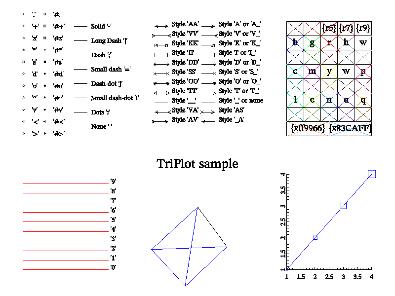
Next: quality2 sample, Previous: quality0 sample, Up: All samples [Contents][Index]
Show all kind of primitives in quality=1.
MGL code:
quality 1
subplot 3 2 0:define y 0.95
define d 0.3:define x0 0.2:define x1 0.5:define x2 0.6
line x0 1-0*d x1 1-0*d 'k-':text x2 y-0*d 'Solid `-`' ':rL'
line x0 1-1*d x1 1-1*d 'k|':text x2 y-1*d 'Long Dash `|`' ':rL'
line x0 1-2*d x1 1-2*d 'k;':text x2 y-2*d 'Dash 1;`' ':rL'
line x0 1-3*d x1 1-3*d 'k=':text x2 y-3*d 'Small dash `=`' ':rL'
line x0 1-4*d x1 1-4*d 'kj':text x2 y-4*d 'Dash-dot `j`' ':rL'
line x0 1-5*d x1 1-5*d 'ki':text x2 y-5*d 'Small dash-dot `i`' ':rL'
line x0 1-6*d x1 1-6*d 'k:':text x2 y-6*d 'Dots `:`' ':rL'
line x0 1-7*d x1 1-7*d 'k ':text x2 y-7*d 'None ``' ':rL'
define d 0.25:define x0 -0.8:define x1 -1:define x2 -0.05
ball x1 5*d 'k.':text x0 5*d '.' ':rL'
ball x1 4*d 'k+':text x0 4*d '+' ':rL'
ball x1 3*d 'kx':text x0 3*d 'x' ':rL'
ball x1 2*d 'k*':text x0 2*d '*' ':rL'
ball x1 d 'ks':text x0 d 's' ':rL'
ball x1 0 'kd':text x0 0 'd' ':rL'
ball x1 -d 0 'ko':text x0 y-d 'o' ':rL'
ball x1 -2*d 0 'k^':text x0 -2*d '\^' ':rL'
ball x1 -3*d 0 'kv':text x0 -3*d 'v' ':rL'
ball x1 -4*d 0 'k<':text x0 -4*d '<' ':rL'
ball x1 -5*d 0 'k>':text x0 -5*d '>' ':rL'
define x0 -0.3:define x1 -0.5
ball x1 5*d 'k#.':text x0 5*d '\#.' ':rL'
ball x1 4*d 'k#+':text x0 4*d '\#+' ':rL'
ball x1 3*d 'k#x':text x0 3*d '\#x' ':rL'
ball x1 2*d 'k#*':text x0 2*d '\#*' ':rL'
ball x1 d 'k#s':text x0 d '\#s' ':rL'
ball x1 0 'k#d':text x0 0 '\#d' ':rL'
ball x1 -d 0 'k#o':text x0 -d '\#o' ':rL'
ball x1 -2*d 0 'k#^':text x0 -2*d '\#\^' ':rL'
ball x1 -3*d 0 'k#v':text x0 -3*d '\#v' ':rL'
ball x1 -4*d 0 'k#<':text x0 -4*d '\#<' ':rL'
ball x1 -5*d 0 'k#>':text x0 -5*d '\#>' ':rL'
subplot 3 2 1
define a 0.1:define b 0.4:define c 0.5
line a 1 b 1 'k-A':text c 1 'Style `A` or `A\_`' ':rL'
line a 0.8 b 0.8 'k-V':text c 0.8 'Style `V` or `V\_`' ':rL'
line a 0.6 b 0.6 'k-K':text c 0.6 'Style `K` or `K\_`' ':rL'
line a 0.4 b 0.4 'k-I':text c 0.4 'Style `I` or `I\_`' ':rL'
line a 0.2 b 0.2 'k-D':text c 0.2 'Style `D` or `D\_`' ':rL'
line a 0 b 0 'k-S':text c 0 'Style `S` or `S\_`' ':rL'
line a -0.2 b -0.2 'k-O':text c -0.2 'Style `O` or `O\_`' ':rL'
line a -0.4 b -0.4 'k-T':text c -0.4 'Style `T` or `T\_`' ':rL'
line a -0.6 b -0.6 'k-_':text c -0.6 'Style `\_` or none' ':rL'
line a -0.8 b -0.8 'k-AS':text c -0.8 'Style `AS`' ':rL'
line a -1 b -1 'k-_A':text c -1 'Style `\_A`' ':rL'
define a -1:define b -0.7:define c -0.6
line a 1 b 1 'kAA':text c 1 'Style `AA`' ':rL'
line a 0.8 b 0.8 'kVV':text c 0.8 'Style `VV`' ':rL'
line a 0.6 b 0.6 'kKK':text c 0.6 'Style `KK`' ':rL'
line a 0.4 b 0.4 'kII':text c 0.4 'Style `II`' ':rL'
line a 0.2 b 0.2 'kDD':text c 0.2 'Style `DD`' ':rL'
line a 0 b 0 'kSS':text c 0 'Style `SS`' ':rL'
line a -0.2 b -0.2 'kOO':text c -0.2 'Style `OO`' ':rL'
line a -0.4 b -0.4 'kTT':text c -0.4 'Style `TT`' ':rL'
line a -0.6 b -0.6 'k-__':text c -0.6 'Style `\_\_`' ':rL'
line a -0.8 b -0.8 'k-VA':text c -0.8 'Style `VA`' ':rL'
line a -1 b -1 'k-AV':text c -1 'Style `AV`' ':rL'
subplot 3 2 2
#LENUQ
facez -1 -1 0 0.4 0.3 'L#':text -0.8 -0.9 'L' 'w:C' -1.4
facez -0.6 -1 0 0.4 0.3 'E#':text -0.4 -0.9 'E' 'w:C' -1.4
facez -0.2 -1 0 0.4 0.3 'N#':text 0 -0.9 'N' 'w:C' -1.4
facez 0.2 -1 0 0.4 0.3 'U#':text 0.4 -0.9 'U' 'w:C' -1.4
facez 0.6 -1 0 0.4 0.3 'Q#':text 0.8 -0.9 'Q' 'w:C' -1.4
#lenuq
facez -1 -0.7 0 0.4 0.3 'l#':text -0.8 -0.6 'l' 'k:C' -1.4
facez -0.6 -0.7 0 0.4 0.3 'e#':text -0.4 -0.6 'e' 'k:C' -1.4
facez -0.2 -0.7 0 0.4 0.3 'n#':text 0 -0.6 'n' 'k:C' -1.4
facez 0.2 -0.7 0 0.4 0.3 'u#':text 0.4 -0.6 'u' 'k:C' -1.4
facez 0.6 -0.7 0 0.4 0.3 'q#':text 0.8 -0.6 'q' 'k:C' -1.4
#CMYkP
facez -1 -0.4 0 0.4 0.3 'C#':text -0.8 -0.3 'C' 'w:C' -1.4
facez -0.6 -0.4 0 0.4 0.3 'M#':text -0.4 -0.3 'M' 'w:C' -1.4
facez -0.2 -0.4 0 0.4 0.3 'Y#':text 0 -0.3 'Y' 'w:C' -1.4
facez 0.2 -0.4 0 0.4 0.3 'k#':text 0.4 -0.3 'k' 'w:C' -1.4
facez 0.6 -0.4 0 0.4 0.3 'P#':text 0.8 -0.3 'P' 'w:C' -1.4
#cmywp
facez -1 -0.1 0 0.4 0.3 'c#':text -0.8 0 'c' 'k:C' -1.4
facez -0.6 -0.1 0 0.4 0.3 'm#':text -0.4 0 'm' 'k:C' -1.4
facez -0.2 -0.1 0 0.4 0.3 'y#':text 0 0 'y' 'k:C' -1.4
facez 0.2 -0.1 0 0.4 0.3 'w#':text 0.4 0 'w' 'k:C' -1.4
facez 0.6 -0.1 0 0.4 0.3 'p#':text 0.8 0 'p' 'k:C' -1.4
#BGRHW
facez -1 0.2 0 0.4 0.3 'B#':text -0.8 0.3 'B' 'w:C' -1.4
facez -0.6 0.2 0 0.4 0.3 'G#':text -0.4 0.3 'G' 'w:C' -1.4
facez -0.2 0.2 0 0.4 0.3 'R#':text 0 0.3 'R' 'w:C' -1.4
facez 0.2 0.2 0 0.4 0.3 'H#':text 0.4 0.3 'H' 'w:C' -1.4
facez 0.6 0.2 0 0.4 0.3 'W#':text 0.8 0.3 'W' 'w:C' -1.4
#bgrhw
facez -1 0.5 0 0.4 0.3 'b#':text -0.8 0.6 'b' 'k:C' -1.4
facez -0.6 0.5 0 0.4 0.3 'g#':text -0.4 0.6 'g' 'k:C' -1.4
facez -0.2 0.5 0 0.4 0.3 'r#':text 0 0.6 'r' 'k:C' -1.4
facez 0.2 0.5 0 0.4 0.3 'h#':text 0.4 0.6 'h' 'k:C' -1.4
facez 0.6 0.5 0 0.4 0.3 'w#':text 0.8 0.6 'w' 'k:C' -1.4
#brighted
facez -1 0.8 0 0.4 0.3 '{r1}#':text -0.8 0.9 '\{r1\}' 'w:C' -1.4
facez -0.6 0.8 0 0.4 0.3 '{r3}#':text -0.4 0.9 '\{r3\}' 'w:C' -1.4
facez -0.2 0.8 0 0.4 0.3 '{r5}#':text 0 0.9 '\{r5\}' 'k:C' -1.4
facez 0.2 0.8 0 0.4 0.3 '{r7}#':text 0.4 0.9 '\{r7\}' 'k:C' -1.4
facez 0.6 0.8 0 0.4 0.3 '{r9}#':text 0.8 0.9 '\{r9\}' 'k:C' -1.4
# HEX
facez -1 -1.3 0 1 0.3 '{xff9966}#':text -0.5 -1.2 '\{xff9966\}' 'k:C' -1.4
facez 0 -1.3 0 1 0.3 '{x83CAFF}#':text 0.5 -1.2 '\{x83caff\}' 'k:C' -1.4
subplot 3 2 3
for $i 0 9
line -1 0.2*$i-1 1 0.2*$i-1 'r','0'+$i
text 1.05 0.2*$i-1 '0'+$i ':L'
next
subplot 3 2 4:title 'TriPlot sample':rotate 50 60
list tt 0 1 2 | 0 1 3 | 0 2 3 | 1 2 3
list xt -1 1 0 0:list yt -1 -1 1 0:list zt -1 -1 -1 1:light on
triplot tt xt yt zt 'b':triplot tt xt yt zt 'k#'
subplot 3 2 5:new r 4 'i+1':ranges 1 4 1 4
axis:mark r r 's':plot r 'b'
C++ code:
void smgl_quality1(mglGraph *gr) // test file export
{
gr->SetQuality(1); all_prims(gr);
}

Next: quality4 sample, Previous: quality1 sample, Up: All samples [Contents][Index]
Show all kind of primitives in quality=2.
MGL code:
quality 2
subplot 3 2 0:define y 0.95
define d 0.3:define x0 0.2:define x1 0.5:define x2 0.6
line x0 1-0*d x1 1-0*d 'k-':text x2 y-0*d 'Solid `-`' ':rL'
line x0 1-1*d x1 1-1*d 'k|':text x2 y-1*d 'Long Dash `|`' ':rL'
line x0 1-2*d x1 1-2*d 'k;':text x2 y-2*d 'Dash 1;`' ':rL'
line x0 1-3*d x1 1-3*d 'k=':text x2 y-3*d 'Small dash `=`' ':rL'
line x0 1-4*d x1 1-4*d 'kj':text x2 y-4*d 'Dash-dot `j`' ':rL'
line x0 1-5*d x1 1-5*d 'ki':text x2 y-5*d 'Small dash-dot `i`' ':rL'
line x0 1-6*d x1 1-6*d 'k:':text x2 y-6*d 'Dots `:`' ':rL'
line x0 1-7*d x1 1-7*d 'k ':text x2 y-7*d 'None ``' ':rL'
define d 0.25:define x0 -0.8:define x1 -1:define x2 -0.05
ball x1 5*d 'k.':text x0 5*d '.' ':rL'
ball x1 4*d 'k+':text x0 4*d '+' ':rL'
ball x1 3*d 'kx':text x0 3*d 'x' ':rL'
ball x1 2*d 'k*':text x0 2*d '*' ':rL'
ball x1 d 'ks':text x0 d 's' ':rL'
ball x1 0 'kd':text x0 0 'd' ':rL'
ball x1 -d 0 'ko':text x0 y-d 'o' ':rL'
ball x1 -2*d 0 'k^':text x0 -2*d '\^' ':rL'
ball x1 -3*d 0 'kv':text x0 -3*d 'v' ':rL'
ball x1 -4*d 0 'k<':text x0 -4*d '<' ':rL'
ball x1 -5*d 0 'k>':text x0 -5*d '>' ':rL'
define x0 -0.3:define x1 -0.5
ball x1 5*d 'k#.':text x0 5*d '\#.' ':rL'
ball x1 4*d 'k#+':text x0 4*d '\#+' ':rL'
ball x1 3*d 'k#x':text x0 3*d '\#x' ':rL'
ball x1 2*d 'k#*':text x0 2*d '\#*' ':rL'
ball x1 d 'k#s':text x0 d '\#s' ':rL'
ball x1 0 'k#d':text x0 0 '\#d' ':rL'
ball x1 -d 0 'k#o':text x0 -d '\#o' ':rL'
ball x1 -2*d 0 'k#^':text x0 -2*d '\#\^' ':rL'
ball x1 -3*d 0 'k#v':text x0 -3*d '\#v' ':rL'
ball x1 -4*d 0 'k#<':text x0 -4*d '\#<' ':rL'
ball x1 -5*d 0 'k#>':text x0 -5*d '\#>' ':rL'
subplot 3 2 1
define a 0.1:define b 0.4:define c 0.5
line a 1 b 1 'k-A':text c 1 'Style `A` or `A\_`' ':rL'
line a 0.8 b 0.8 'k-V':text c 0.8 'Style `V` or `V\_`' ':rL'
line a 0.6 b 0.6 'k-K':text c 0.6 'Style `K` or `K\_`' ':rL'
line a 0.4 b 0.4 'k-I':text c 0.4 'Style `I` or `I\_`' ':rL'
line a 0.2 b 0.2 'k-D':text c 0.2 'Style `D` or `D\_`' ':rL'
line a 0 b 0 'k-S':text c 0 'Style `S` or `S\_`' ':rL'
line a -0.2 b -0.2 'k-O':text c -0.2 'Style `O` or `O\_`' ':rL'
line a -0.4 b -0.4 'k-T':text c -0.4 'Style `T` or `T\_`' ':rL'
line a -0.6 b -0.6 'k-_':text c -0.6 'Style `\_` or none' ':rL'
line a -0.8 b -0.8 'k-AS':text c -0.8 'Style `AS`' ':rL'
line a -1 b -1 'k-_A':text c -1 'Style `\_A`' ':rL'
define a -1:define b -0.7:define c -0.6
line a 1 b 1 'kAA':text c 1 'Style `AA`' ':rL'
line a 0.8 b 0.8 'kVV':text c 0.8 'Style `VV`' ':rL'
line a 0.6 b 0.6 'kKK':text c 0.6 'Style `KK`' ':rL'
line a 0.4 b 0.4 'kII':text c 0.4 'Style `II`' ':rL'
line a 0.2 b 0.2 'kDD':text c 0.2 'Style `DD`' ':rL'
line a 0 b 0 'kSS':text c 0 'Style `SS`' ':rL'
line a -0.2 b -0.2 'kOO':text c -0.2 'Style `OO`' ':rL'
line a -0.4 b -0.4 'kTT':text c -0.4 'Style `TT`' ':rL'
line a -0.6 b -0.6 'k-__':text c -0.6 'Style `\_\_`' ':rL'
line a -0.8 b -0.8 'k-VA':text c -0.8 'Style `VA`' ':rL'
line a -1 b -1 'k-AV':text c -1 'Style `AV`' ':rL'
subplot 3 2 2
#LENUQ
facez -1 -1 0 0.4 0.3 'L#':text -0.8 -0.9 'L' 'w:C' -1.4
facez -0.6 -1 0 0.4 0.3 'E#':text -0.4 -0.9 'E' 'w:C' -1.4
facez -0.2 -1 0 0.4 0.3 'N#':text 0 -0.9 'N' 'w:C' -1.4
facez 0.2 -1 0 0.4 0.3 'U#':text 0.4 -0.9 'U' 'w:C' -1.4
facez 0.6 -1 0 0.4 0.3 'Q#':text 0.8 -0.9 'Q' 'w:C' -1.4
#lenuq
facez -1 -0.7 0 0.4 0.3 'l#':text -0.8 -0.6 'l' 'k:C' -1.4
facez -0.6 -0.7 0 0.4 0.3 'e#':text -0.4 -0.6 'e' 'k:C' -1.4
facez -0.2 -0.7 0 0.4 0.3 'n#':text 0 -0.6 'n' 'k:C' -1.4
facez 0.2 -0.7 0 0.4 0.3 'u#':text 0.4 -0.6 'u' 'k:C' -1.4
facez 0.6 -0.7 0 0.4 0.3 'q#':text 0.8 -0.6 'q' 'k:C' -1.4
#CMYkP
facez -1 -0.4 0 0.4 0.3 'C#':text -0.8 -0.3 'C' 'w:C' -1.4
facez -0.6 -0.4 0 0.4 0.3 'M#':text -0.4 -0.3 'M' 'w:C' -1.4
facez -0.2 -0.4 0 0.4 0.3 'Y#':text 0 -0.3 'Y' 'w:C' -1.4
facez 0.2 -0.4 0 0.4 0.3 'k#':text 0.4 -0.3 'k' 'w:C' -1.4
facez 0.6 -0.4 0 0.4 0.3 'P#':text 0.8 -0.3 'P' 'w:C' -1.4
#cmywp
facez -1 -0.1 0 0.4 0.3 'c#':text -0.8 0 'c' 'k:C' -1.4
facez -0.6 -0.1 0 0.4 0.3 'm#':text -0.4 0 'm' 'k:C' -1.4
facez -0.2 -0.1 0 0.4 0.3 'y#':text 0 0 'y' 'k:C' -1.4
facez 0.2 -0.1 0 0.4 0.3 'w#':text 0.4 0 'w' 'k:C' -1.4
facez 0.6 -0.1 0 0.4 0.3 'p#':text 0.8 0 'p' 'k:C' -1.4
#BGRHW
facez -1 0.2 0 0.4 0.3 'B#':text -0.8 0.3 'B' 'w:C' -1.4
facez -0.6 0.2 0 0.4 0.3 'G#':text -0.4 0.3 'G' 'w:C' -1.4
facez -0.2 0.2 0 0.4 0.3 'R#':text 0 0.3 'R' 'w:C' -1.4
facez 0.2 0.2 0 0.4 0.3 'H#':text 0.4 0.3 'H' 'w:C' -1.4
facez 0.6 0.2 0 0.4 0.3 'W#':text 0.8 0.3 'W' 'w:C' -1.4
#bgrhw
facez -1 0.5 0 0.4 0.3 'b#':text -0.8 0.6 'b' 'k:C' -1.4
facez -0.6 0.5 0 0.4 0.3 'g#':text -0.4 0.6 'g' 'k:C' -1.4
facez -0.2 0.5 0 0.4 0.3 'r#':text 0 0.6 'r' 'k:C' -1.4
facez 0.2 0.5 0 0.4 0.3 'h#':text 0.4 0.6 'h' 'k:C' -1.4
facez 0.6 0.5 0 0.4 0.3 'w#':text 0.8 0.6 'w' 'k:C' -1.4
#brighted
facez -1 0.8 0 0.4 0.3 '{r1}#':text -0.8 0.9 '\{r1\}' 'w:C' -1.4
facez -0.6 0.8 0 0.4 0.3 '{r3}#':text -0.4 0.9 '\{r3\}' 'w:C' -1.4
facez -0.2 0.8 0 0.4 0.3 '{r5}#':text 0 0.9 '\{r5\}' 'k:C' -1.4
facez 0.2 0.8 0 0.4 0.3 '{r7}#':text 0.4 0.9 '\{r7\}' 'k:C' -1.4
facez 0.6 0.8 0 0.4 0.3 '{r9}#':text 0.8 0.9 '\{r9\}' 'k:C' -1.4
# HEX
facez -1 -1.3 0 1 0.3 '{xff9966}#':text -0.5 -1.2 '\{xff9966\}' 'k:C' -1.4
facez 0 -1.3 0 1 0.3 '{x83CAFF}#':text 0.5 -1.2 '\{x83caff\}' 'k:C' -1.4
subplot 3 2 3
for $i 0 9
line -1 0.2*$i-1 1 0.2*$i-1 'r','0'+$i
text 1.05 0.2*$i-1 '0'+$i ':L'
next
subplot 3 2 4:title 'TriPlot sample':rotate 50 60
list tt 0 1 2 | 0 1 3 | 0 2 3 | 1 2 3
list xt -1 1 0 0:list yt -1 -1 1 0:list zt -1 -1 -1 1:light on
triplot tt xt yt zt 'b':triplot tt xt yt zt 'k#'
subplot 3 2 5:new r 4 'i+1':ranges 1 4 1 4
axis:mark r r 's':plot r 'b'
C++ code:
void smgl_quality2(mglGraph *gr) // test file export
{
gr->SetQuality(2); all_prims(gr);
}
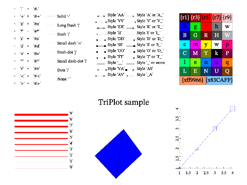
Next: quality5 sample, Previous: quality2 sample, Up: All samples [Contents][Index]
Show all kind of primitives in quality=4.
MGL code:
quality 4
subplot 3 2 0:define y 0.95
define d 0.3:define x0 0.2:define x1 0.5:define x2 0.6
line x0 1-0*d x1 1-0*d 'k-':text x2 y-0*d 'Solid `-`' ':rL'
line x0 1-1*d x1 1-1*d 'k|':text x2 y-1*d 'Long Dash `|`' ':rL'
line x0 1-2*d x1 1-2*d 'k;':text x2 y-2*d 'Dash 1;`' ':rL'
line x0 1-3*d x1 1-3*d 'k=':text x2 y-3*d 'Small dash `=`' ':rL'
line x0 1-4*d x1 1-4*d 'kj':text x2 y-4*d 'Dash-dot `j`' ':rL'
line x0 1-5*d x1 1-5*d 'ki':text x2 y-5*d 'Small dash-dot `i`' ':rL'
line x0 1-6*d x1 1-6*d 'k:':text x2 y-6*d 'Dots `:`' ':rL'
line x0 1-7*d x1 1-7*d 'k ':text x2 y-7*d 'None ``' ':rL'
define d 0.25:define x0 -0.8:define x1 -1:define x2 -0.05
ball x1 5*d 'k.':text x0 5*d '.' ':rL'
ball x1 4*d 'k+':text x0 4*d '+' ':rL'
ball x1 3*d 'kx':text x0 3*d 'x' ':rL'
ball x1 2*d 'k*':text x0 2*d '*' ':rL'
ball x1 d 'ks':text x0 d 's' ':rL'
ball x1 0 'kd':text x0 0 'd' ':rL'
ball x1 -d 0 'ko':text x0 y-d 'o' ':rL'
ball x1 -2*d 0 'k^':text x0 -2*d '\^' ':rL'
ball x1 -3*d 0 'kv':text x0 -3*d 'v' ':rL'
ball x1 -4*d 0 'k<':text x0 -4*d '<' ':rL'
ball x1 -5*d 0 'k>':text x0 -5*d '>' ':rL'
define x0 -0.3:define x1 -0.5
ball x1 5*d 'k#.':text x0 5*d '\#.' ':rL'
ball x1 4*d 'k#+':text x0 4*d '\#+' ':rL'
ball x1 3*d 'k#x':text x0 3*d '\#x' ':rL'
ball x1 2*d 'k#*':text x0 2*d '\#*' ':rL'
ball x1 d 'k#s':text x0 d '\#s' ':rL'
ball x1 0 'k#d':text x0 0 '\#d' ':rL'
ball x1 -d 0 'k#o':text x0 -d '\#o' ':rL'
ball x1 -2*d 0 'k#^':text x0 -2*d '\#\^' ':rL'
ball x1 -3*d 0 'k#v':text x0 -3*d '\#v' ':rL'
ball x1 -4*d 0 'k#<':text x0 -4*d '\#<' ':rL'
ball x1 -5*d 0 'k#>':text x0 -5*d '\#>' ':rL'
subplot 3 2 1
define a 0.1:define b 0.4:define c 0.5
line a 1 b 1 'k-A':text c 1 'Style `A` or `A\_`' ':rL'
line a 0.8 b 0.8 'k-V':text c 0.8 'Style `V` or `V\_`' ':rL'
line a 0.6 b 0.6 'k-K':text c 0.6 'Style `K` or `K\_`' ':rL'
line a 0.4 b 0.4 'k-I':text c 0.4 'Style `I` or `I\_`' ':rL'
line a 0.2 b 0.2 'k-D':text c 0.2 'Style `D` or `D\_`' ':rL'
line a 0 b 0 'k-S':text c 0 'Style `S` or `S\_`' ':rL'
line a -0.2 b -0.2 'k-O':text c -0.2 'Style `O` or `O\_`' ':rL'
line a -0.4 b -0.4 'k-T':text c -0.4 'Style `T` or `T\_`' ':rL'
line a -0.6 b -0.6 'k-_':text c -0.6 'Style `\_` or none' ':rL'
line a -0.8 b -0.8 'k-AS':text c -0.8 'Style `AS`' ':rL'
line a -1 b -1 'k-_A':text c -1 'Style `\_A`' ':rL'
define a -1:define b -0.7:define c -0.6
line a 1 b 1 'kAA':text c 1 'Style `AA`' ':rL'
line a 0.8 b 0.8 'kVV':text c 0.8 'Style `VV`' ':rL'
line a 0.6 b 0.6 'kKK':text c 0.6 'Style `KK`' ':rL'
line a 0.4 b 0.4 'kII':text c 0.4 'Style `II`' ':rL'
line a 0.2 b 0.2 'kDD':text c 0.2 'Style `DD`' ':rL'
line a 0 b 0 'kSS':text c 0 'Style `SS`' ':rL'
line a -0.2 b -0.2 'kOO':text c -0.2 'Style `OO`' ':rL'
line a -0.4 b -0.4 'kTT':text c -0.4 'Style `TT`' ':rL'
line a -0.6 b -0.6 'k-__':text c -0.6 'Style `\_\_`' ':rL'
line a -0.8 b -0.8 'k-VA':text c -0.8 'Style `VA`' ':rL'
line a -1 b -1 'k-AV':text c -1 'Style `AV`' ':rL'
subplot 3 2 2
#LENUQ
facez -1 -1 0 0.4 0.3 'L#':text -0.8 -0.9 'L' 'w:C' -1.4
facez -0.6 -1 0 0.4 0.3 'E#':text -0.4 -0.9 'E' 'w:C' -1.4
facez -0.2 -1 0 0.4 0.3 'N#':text 0 -0.9 'N' 'w:C' -1.4
facez 0.2 -1 0 0.4 0.3 'U#':text 0.4 -0.9 'U' 'w:C' -1.4
facez 0.6 -1 0 0.4 0.3 'Q#':text 0.8 -0.9 'Q' 'w:C' -1.4
#lenuq
facez -1 -0.7 0 0.4 0.3 'l#':text -0.8 -0.6 'l' 'k:C' -1.4
facez -0.6 -0.7 0 0.4 0.3 'e#':text -0.4 -0.6 'e' 'k:C' -1.4
facez -0.2 -0.7 0 0.4 0.3 'n#':text 0 -0.6 'n' 'k:C' -1.4
facez 0.2 -0.7 0 0.4 0.3 'u#':text 0.4 -0.6 'u' 'k:C' -1.4
facez 0.6 -0.7 0 0.4 0.3 'q#':text 0.8 -0.6 'q' 'k:C' -1.4
#CMYkP
facez -1 -0.4 0 0.4 0.3 'C#':text -0.8 -0.3 'C' 'w:C' -1.4
facez -0.6 -0.4 0 0.4 0.3 'M#':text -0.4 -0.3 'M' 'w:C' -1.4
facez -0.2 -0.4 0 0.4 0.3 'Y#':text 0 -0.3 'Y' 'w:C' -1.4
facez 0.2 -0.4 0 0.4 0.3 'k#':text 0.4 -0.3 'k' 'w:C' -1.4
facez 0.6 -0.4 0 0.4 0.3 'P#':text 0.8 -0.3 'P' 'w:C' -1.4
#cmywp
facez -1 -0.1 0 0.4 0.3 'c#':text -0.8 0 'c' 'k:C' -1.4
facez -0.6 -0.1 0 0.4 0.3 'm#':text -0.4 0 'm' 'k:C' -1.4
facez -0.2 -0.1 0 0.4 0.3 'y#':text 0 0 'y' 'k:C' -1.4
facez 0.2 -0.1 0 0.4 0.3 'w#':text 0.4 0 'w' 'k:C' -1.4
facez 0.6 -0.1 0 0.4 0.3 'p#':text 0.8 0 'p' 'k:C' -1.4
#BGRHW
facez -1 0.2 0 0.4 0.3 'B#':text -0.8 0.3 'B' 'w:C' -1.4
facez -0.6 0.2 0 0.4 0.3 'G#':text -0.4 0.3 'G' 'w:C' -1.4
facez -0.2 0.2 0 0.4 0.3 'R#':text 0 0.3 'R' 'w:C' -1.4
facez 0.2 0.2 0 0.4 0.3 'H#':text 0.4 0.3 'H' 'w:C' -1.4
facez 0.6 0.2 0 0.4 0.3 'W#':text 0.8 0.3 'W' 'w:C' -1.4
#bgrhw
facez -1 0.5 0 0.4 0.3 'b#':text -0.8 0.6 'b' 'k:C' -1.4
facez -0.6 0.5 0 0.4 0.3 'g#':text -0.4 0.6 'g' 'k:C' -1.4
facez -0.2 0.5 0 0.4 0.3 'r#':text 0 0.6 'r' 'k:C' -1.4
facez 0.2 0.5 0 0.4 0.3 'h#':text 0.4 0.6 'h' 'k:C' -1.4
facez 0.6 0.5 0 0.4 0.3 'w#':text 0.8 0.6 'w' 'k:C' -1.4
#brighted
facez -1 0.8 0 0.4 0.3 '{r1}#':text -0.8 0.9 '\{r1\}' 'w:C' -1.4
facez -0.6 0.8 0 0.4 0.3 '{r3}#':text -0.4 0.9 '\{r3\}' 'w:C' -1.4
facez -0.2 0.8 0 0.4 0.3 '{r5}#':text 0 0.9 '\{r5\}' 'k:C' -1.4
facez 0.2 0.8 0 0.4 0.3 '{r7}#':text 0.4 0.9 '\{r7\}' 'k:C' -1.4
facez 0.6 0.8 0 0.4 0.3 '{r9}#':text 0.8 0.9 '\{r9\}' 'k:C' -1.4
# HEX
facez -1 -1.3 0 1 0.3 '{xff9966}#':text -0.5 -1.2 '\{xff9966\}' 'k:C' -1.4
facez 0 -1.3 0 1 0.3 '{x83CAFF}#':text 0.5 -1.2 '\{x83caff\}' 'k:C' -1.4
subplot 3 2 3
for $i 0 9
line -1 0.2*$i-1 1 0.2*$i-1 'r','0'+$i
text 1.05 0.2*$i-1 '0'+$i ':L'
next
subplot 3 2 4:title 'TriPlot sample':rotate 50 60
list tt 0 1 2 | 0 1 3 | 0 2 3 | 1 2 3
list xt -1 1 0 0:list yt -1 -1 1 0:list zt -1 -1 -1 1:light on
triplot tt xt yt zt 'b':triplot tt xt yt zt 'k#'
subplot 3 2 5:new r 4 'i+1':ranges 1 4 1 4
axis:mark r r 's':plot r 'b'
C++ code:
void smgl_quality4(mglGraph *gr) // test file export
{
gr->SetQuality(4); all_prims(gr);
}
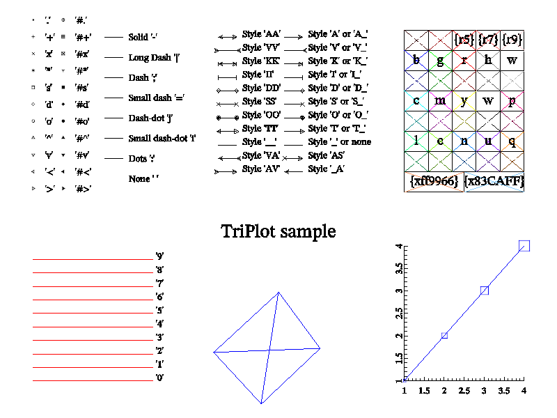
Next: quality6 sample, Previous: quality4 sample, Up: All samples [Contents][Index]
Show all kind of primitives in quality=5.
MGL code:
quality 5
subplot 3 2 0:define y 0.95
define d 0.3:define x0 0.2:define x1 0.5:define x2 0.6
line x0 1-0*d x1 1-0*d 'k-':text x2 y-0*d 'Solid `-`' ':rL'
line x0 1-1*d x1 1-1*d 'k|':text x2 y-1*d 'Long Dash `|`' ':rL'
line x0 1-2*d x1 1-2*d 'k;':text x2 y-2*d 'Dash 1;`' ':rL'
line x0 1-3*d x1 1-3*d 'k=':text x2 y-3*d 'Small dash `=`' ':rL'
line x0 1-4*d x1 1-4*d 'kj':text x2 y-4*d 'Dash-dot `j`' ':rL'
line x0 1-5*d x1 1-5*d 'ki':text x2 y-5*d 'Small dash-dot `i`' ':rL'
line x0 1-6*d x1 1-6*d 'k:':text x2 y-6*d 'Dots `:`' ':rL'
line x0 1-7*d x1 1-7*d 'k ':text x2 y-7*d 'None ``' ':rL'
define d 0.25:define x0 -0.8:define x1 -1:define x2 -0.05
ball x1 5*d 'k.':text x0 5*d '.' ':rL'
ball x1 4*d 'k+':text x0 4*d '+' ':rL'
ball x1 3*d 'kx':text x0 3*d 'x' ':rL'
ball x1 2*d 'k*':text x0 2*d '*' ':rL'
ball x1 d 'ks':text x0 d 's' ':rL'
ball x1 0 'kd':text x0 0 'd' ':rL'
ball x1 -d 0 'ko':text x0 y-d 'o' ':rL'
ball x1 -2*d 0 'k^':text x0 -2*d '\^' ':rL'
ball x1 -3*d 0 'kv':text x0 -3*d 'v' ':rL'
ball x1 -4*d 0 'k<':text x0 -4*d '<' ':rL'
ball x1 -5*d 0 'k>':text x0 -5*d '>' ':rL'
define x0 -0.3:define x1 -0.5
ball x1 5*d 'k#.':text x0 5*d '\#.' ':rL'
ball x1 4*d 'k#+':text x0 4*d '\#+' ':rL'
ball x1 3*d 'k#x':text x0 3*d '\#x' ':rL'
ball x1 2*d 'k#*':text x0 2*d '\#*' ':rL'
ball x1 d 'k#s':text x0 d '\#s' ':rL'
ball x1 0 'k#d':text x0 0 '\#d' ':rL'
ball x1 -d 0 'k#o':text x0 -d '\#o' ':rL'
ball x1 -2*d 0 'k#^':text x0 -2*d '\#\^' ':rL'
ball x1 -3*d 0 'k#v':text x0 -3*d '\#v' ':rL'
ball x1 -4*d 0 'k#<':text x0 -4*d '\#<' ':rL'
ball x1 -5*d 0 'k#>':text x0 -5*d '\#>' ':rL'
subplot 3 2 1
define a 0.1:define b 0.4:define c 0.5
line a 1 b 1 'k-A':text c 1 'Style `A` or `A\_`' ':rL'
line a 0.8 b 0.8 'k-V':text c 0.8 'Style `V` or `V\_`' ':rL'
line a 0.6 b 0.6 'k-K':text c 0.6 'Style `K` or `K\_`' ':rL'
line a 0.4 b 0.4 'k-I':text c 0.4 'Style `I` or `I\_`' ':rL'
line a 0.2 b 0.2 'k-D':text c 0.2 'Style `D` or `D\_`' ':rL'
line a 0 b 0 'k-S':text c 0 'Style `S` or `S\_`' ':rL'
line a -0.2 b -0.2 'k-O':text c -0.2 'Style `O` or `O\_`' ':rL'
line a -0.4 b -0.4 'k-T':text c -0.4 'Style `T` or `T\_`' ':rL'
line a -0.6 b -0.6 'k-_':text c -0.6 'Style `\_` or none' ':rL'
line a -0.8 b -0.8 'k-AS':text c -0.8 'Style `AS`' ':rL'
line a -1 b -1 'k-_A':text c -1 'Style `\_A`' ':rL'
define a -1:define b -0.7:define c -0.6
line a 1 b 1 'kAA':text c 1 'Style `AA`' ':rL'
line a 0.8 b 0.8 'kVV':text c 0.8 'Style `VV`' ':rL'
line a 0.6 b 0.6 'kKK':text c 0.6 'Style `KK`' ':rL'
line a 0.4 b 0.4 'kII':text c 0.4 'Style `II`' ':rL'
line a 0.2 b 0.2 'kDD':text c 0.2 'Style `DD`' ':rL'
line a 0 b 0 'kSS':text c 0 'Style `SS`' ':rL'
line a -0.2 b -0.2 'kOO':text c -0.2 'Style `OO`' ':rL'
line a -0.4 b -0.4 'kTT':text c -0.4 'Style `TT`' ':rL'
line a -0.6 b -0.6 'k-__':text c -0.6 'Style `\_\_`' ':rL'
line a -0.8 b -0.8 'k-VA':text c -0.8 'Style `VA`' ':rL'
line a -1 b -1 'k-AV':text c -1 'Style `AV`' ':rL'
subplot 3 2 2
#LENUQ
facez -1 -1 0 0.4 0.3 'L#':text -0.8 -0.9 'L' 'w:C' -1.4
facez -0.6 -1 0 0.4 0.3 'E#':text -0.4 -0.9 'E' 'w:C' -1.4
facez -0.2 -1 0 0.4 0.3 'N#':text 0 -0.9 'N' 'w:C' -1.4
facez 0.2 -1 0 0.4 0.3 'U#':text 0.4 -0.9 'U' 'w:C' -1.4
facez 0.6 -1 0 0.4 0.3 'Q#':text 0.8 -0.9 'Q' 'w:C' -1.4
#lenuq
facez -1 -0.7 0 0.4 0.3 'l#':text -0.8 -0.6 'l' 'k:C' -1.4
facez -0.6 -0.7 0 0.4 0.3 'e#':text -0.4 -0.6 'e' 'k:C' -1.4
facez -0.2 -0.7 0 0.4 0.3 'n#':text 0 -0.6 'n' 'k:C' -1.4
facez 0.2 -0.7 0 0.4 0.3 'u#':text 0.4 -0.6 'u' 'k:C' -1.4
facez 0.6 -0.7 0 0.4 0.3 'q#':text 0.8 -0.6 'q' 'k:C' -1.4
#CMYkP
facez -1 -0.4 0 0.4 0.3 'C#':text -0.8 -0.3 'C' 'w:C' -1.4
facez -0.6 -0.4 0 0.4 0.3 'M#':text -0.4 -0.3 'M' 'w:C' -1.4
facez -0.2 -0.4 0 0.4 0.3 'Y#':text 0 -0.3 'Y' 'w:C' -1.4
facez 0.2 -0.4 0 0.4 0.3 'k#':text 0.4 -0.3 'k' 'w:C' -1.4
facez 0.6 -0.4 0 0.4 0.3 'P#':text 0.8 -0.3 'P' 'w:C' -1.4
#cmywp
facez -1 -0.1 0 0.4 0.3 'c#':text -0.8 0 'c' 'k:C' -1.4
facez -0.6 -0.1 0 0.4 0.3 'm#':text -0.4 0 'm' 'k:C' -1.4
facez -0.2 -0.1 0 0.4 0.3 'y#':text 0 0 'y' 'k:C' -1.4
facez 0.2 -0.1 0 0.4 0.3 'w#':text 0.4 0 'w' 'k:C' -1.4
facez 0.6 -0.1 0 0.4 0.3 'p#':text 0.8 0 'p' 'k:C' -1.4
#BGRHW
facez -1 0.2 0 0.4 0.3 'B#':text -0.8 0.3 'B' 'w:C' -1.4
facez -0.6 0.2 0 0.4 0.3 'G#':text -0.4 0.3 'G' 'w:C' -1.4
facez -0.2 0.2 0 0.4 0.3 'R#':text 0 0.3 'R' 'w:C' -1.4
facez 0.2 0.2 0 0.4 0.3 'H#':text 0.4 0.3 'H' 'w:C' -1.4
facez 0.6 0.2 0 0.4 0.3 'W#':text 0.8 0.3 'W' 'w:C' -1.4
#bgrhw
facez -1 0.5 0 0.4 0.3 'b#':text -0.8 0.6 'b' 'k:C' -1.4
facez -0.6 0.5 0 0.4 0.3 'g#':text -0.4 0.6 'g' 'k:C' -1.4
facez -0.2 0.5 0 0.4 0.3 'r#':text 0 0.6 'r' 'k:C' -1.4
facez 0.2 0.5 0 0.4 0.3 'h#':text 0.4 0.6 'h' 'k:C' -1.4
facez 0.6 0.5 0 0.4 0.3 'w#':text 0.8 0.6 'w' 'k:C' -1.4
#brighted
facez -1 0.8 0 0.4 0.3 '{r1}#':text -0.8 0.9 '\{r1\}' 'w:C' -1.4
facez -0.6 0.8 0 0.4 0.3 '{r3}#':text -0.4 0.9 '\{r3\}' 'w:C' -1.4
facez -0.2 0.8 0 0.4 0.3 '{r5}#':text 0 0.9 '\{r5\}' 'k:C' -1.4
facez 0.2 0.8 0 0.4 0.3 '{r7}#':text 0.4 0.9 '\{r7\}' 'k:C' -1.4
facez 0.6 0.8 0 0.4 0.3 '{r9}#':text 0.8 0.9 '\{r9\}' 'k:C' -1.4
# HEX
facez -1 -1.3 0 1 0.3 '{xff9966}#':text -0.5 -1.2 '\{xff9966\}' 'k:C' -1.4
facez 0 -1.3 0 1 0.3 '{x83CAFF}#':text 0.5 -1.2 '\{x83caff\}' 'k:C' -1.4
subplot 3 2 3
for $i 0 9
line -1 0.2*$i-1 1 0.2*$i-1 'r','0'+$i
text 1.05 0.2*$i-1 '0'+$i ':L'
next
subplot 3 2 4:title 'TriPlot sample':rotate 50 60
list tt 0 1 2 | 0 1 3 | 0 2 3 | 1 2 3
list xt -1 1 0 0:list yt -1 -1 1 0:list zt -1 -1 -1 1:light on
triplot tt xt yt zt 'b':triplot tt xt yt zt 'k#'
subplot 3 2 5:new r 4 'i+1':ranges 1 4 1 4
axis:mark r r 's':plot r 'b'
C++ code:
void smgl_quality5(mglGraph *gr) // test file export
{
gr->SetQuality(5); all_prims(gr);
}

Next: quality8 sample, Previous: quality5 sample, Up: All samples [Contents][Index]
Show all kind of primitives in quality=6.
MGL code:
quality 6
subplot 3 2 0:define y 0.95
define d 0.3:define x0 0.2:define x1 0.5:define x2 0.6
line x0 1-0*d x1 1-0*d 'k-':text x2 y-0*d 'Solid `-`' ':rL'
line x0 1-1*d x1 1-1*d 'k|':text x2 y-1*d 'Long Dash `|`' ':rL'
line x0 1-2*d x1 1-2*d 'k;':text x2 y-2*d 'Dash 1;`' ':rL'
line x0 1-3*d x1 1-3*d 'k=':text x2 y-3*d 'Small dash `=`' ':rL'
line x0 1-4*d x1 1-4*d 'kj':text x2 y-4*d 'Dash-dot `j`' ':rL'
line x0 1-5*d x1 1-5*d 'ki':text x2 y-5*d 'Small dash-dot `i`' ':rL'
line x0 1-6*d x1 1-6*d 'k:':text x2 y-6*d 'Dots `:`' ':rL'
line x0 1-7*d x1 1-7*d 'k ':text x2 y-7*d 'None ``' ':rL'
define d 0.25:define x0 -0.8:define x1 -1:define x2 -0.05
ball x1 5*d 'k.':text x0 5*d '.' ':rL'
ball x1 4*d 'k+':text x0 4*d '+' ':rL'
ball x1 3*d 'kx':text x0 3*d 'x' ':rL'
ball x1 2*d 'k*':text x0 2*d '*' ':rL'
ball x1 d 'ks':text x0 d 's' ':rL'
ball x1 0 'kd':text x0 0 'd' ':rL'
ball x1 -d 0 'ko':text x0 y-d 'o' ':rL'
ball x1 -2*d 0 'k^':text x0 -2*d '\^' ':rL'
ball x1 -3*d 0 'kv':text x0 -3*d 'v' ':rL'
ball x1 -4*d 0 'k<':text x0 -4*d '<' ':rL'
ball x1 -5*d 0 'k>':text x0 -5*d '>' ':rL'
define x0 -0.3:define x1 -0.5
ball x1 5*d 'k#.':text x0 5*d '\#.' ':rL'
ball x1 4*d 'k#+':text x0 4*d '\#+' ':rL'
ball x1 3*d 'k#x':text x0 3*d '\#x' ':rL'
ball x1 2*d 'k#*':text x0 2*d '\#*' ':rL'
ball x1 d 'k#s':text x0 d '\#s' ':rL'
ball x1 0 'k#d':text x0 0 '\#d' ':rL'
ball x1 -d 0 'k#o':text x0 -d '\#o' ':rL'
ball x1 -2*d 0 'k#^':text x0 -2*d '\#\^' ':rL'
ball x1 -3*d 0 'k#v':text x0 -3*d '\#v' ':rL'
ball x1 -4*d 0 'k#<':text x0 -4*d '\#<' ':rL'
ball x1 -5*d 0 'k#>':text x0 -5*d '\#>' ':rL'
subplot 3 2 1
define a 0.1:define b 0.4:define c 0.5
line a 1 b 1 'k-A':text c 1 'Style `A` or `A\_`' ':rL'
line a 0.8 b 0.8 'k-V':text c 0.8 'Style `V` or `V\_`' ':rL'
line a 0.6 b 0.6 'k-K':text c 0.6 'Style `K` or `K\_`' ':rL'
line a 0.4 b 0.4 'k-I':text c 0.4 'Style `I` or `I\_`' ':rL'
line a 0.2 b 0.2 'k-D':text c 0.2 'Style `D` or `D\_`' ':rL'
line a 0 b 0 'k-S':text c 0 'Style `S` or `S\_`' ':rL'
line a -0.2 b -0.2 'k-O':text c -0.2 'Style `O` or `O\_`' ':rL'
line a -0.4 b -0.4 'k-T':text c -0.4 'Style `T` or `T\_`' ':rL'
line a -0.6 b -0.6 'k-_':text c -0.6 'Style `\_` or none' ':rL'
line a -0.8 b -0.8 'k-AS':text c -0.8 'Style `AS`' ':rL'
line a -1 b -1 'k-_A':text c -1 'Style `\_A`' ':rL'
define a -1:define b -0.7:define c -0.6
line a 1 b 1 'kAA':text c 1 'Style `AA`' ':rL'
line a 0.8 b 0.8 'kVV':text c 0.8 'Style `VV`' ':rL'
line a 0.6 b 0.6 'kKK':text c 0.6 'Style `KK`' ':rL'
line a 0.4 b 0.4 'kII':text c 0.4 'Style `II`' ':rL'
line a 0.2 b 0.2 'kDD':text c 0.2 'Style `DD`' ':rL'
line a 0 b 0 'kSS':text c 0 'Style `SS`' ':rL'
line a -0.2 b -0.2 'kOO':text c -0.2 'Style `OO`' ':rL'
line a -0.4 b -0.4 'kTT':text c -0.4 'Style `TT`' ':rL'
line a -0.6 b -0.6 'k-__':text c -0.6 'Style `\_\_`' ':rL'
line a -0.8 b -0.8 'k-VA':text c -0.8 'Style `VA`' ':rL'
line a -1 b -1 'k-AV':text c -1 'Style `AV`' ':rL'
subplot 3 2 2
#LENUQ
facez -1 -1 0 0.4 0.3 'L#':text -0.8 -0.9 'L' 'w:C' -1.4
facez -0.6 -1 0 0.4 0.3 'E#':text -0.4 -0.9 'E' 'w:C' -1.4
facez -0.2 -1 0 0.4 0.3 'N#':text 0 -0.9 'N' 'w:C' -1.4
facez 0.2 -1 0 0.4 0.3 'U#':text 0.4 -0.9 'U' 'w:C' -1.4
facez 0.6 -1 0 0.4 0.3 'Q#':text 0.8 -0.9 'Q' 'w:C' -1.4
#lenuq
facez -1 -0.7 0 0.4 0.3 'l#':text -0.8 -0.6 'l' 'k:C' -1.4
facez -0.6 -0.7 0 0.4 0.3 'e#':text -0.4 -0.6 'e' 'k:C' -1.4
facez -0.2 -0.7 0 0.4 0.3 'n#':text 0 -0.6 'n' 'k:C' -1.4
facez 0.2 -0.7 0 0.4 0.3 'u#':text 0.4 -0.6 'u' 'k:C' -1.4
facez 0.6 -0.7 0 0.4 0.3 'q#':text 0.8 -0.6 'q' 'k:C' -1.4
#CMYkP
facez -1 -0.4 0 0.4 0.3 'C#':text -0.8 -0.3 'C' 'w:C' -1.4
facez -0.6 -0.4 0 0.4 0.3 'M#':text -0.4 -0.3 'M' 'w:C' -1.4
facez -0.2 -0.4 0 0.4 0.3 'Y#':text 0 -0.3 'Y' 'w:C' -1.4
facez 0.2 -0.4 0 0.4 0.3 'k#':text 0.4 -0.3 'k' 'w:C' -1.4
facez 0.6 -0.4 0 0.4 0.3 'P#':text 0.8 -0.3 'P' 'w:C' -1.4
#cmywp
facez -1 -0.1 0 0.4 0.3 'c#':text -0.8 0 'c' 'k:C' -1.4
facez -0.6 -0.1 0 0.4 0.3 'm#':text -0.4 0 'm' 'k:C' -1.4
facez -0.2 -0.1 0 0.4 0.3 'y#':text 0 0 'y' 'k:C' -1.4
facez 0.2 -0.1 0 0.4 0.3 'w#':text 0.4 0 'w' 'k:C' -1.4
facez 0.6 -0.1 0 0.4 0.3 'p#':text 0.8 0 'p' 'k:C' -1.4
#BGRHW
facez -1 0.2 0 0.4 0.3 'B#':text -0.8 0.3 'B' 'w:C' -1.4
facez -0.6 0.2 0 0.4 0.3 'G#':text -0.4 0.3 'G' 'w:C' -1.4
facez -0.2 0.2 0 0.4 0.3 'R#':text 0 0.3 'R' 'w:C' -1.4
facez 0.2 0.2 0 0.4 0.3 'H#':text 0.4 0.3 'H' 'w:C' -1.4
facez 0.6 0.2 0 0.4 0.3 'W#':text 0.8 0.3 'W' 'w:C' -1.4
#bgrhw
facez -1 0.5 0 0.4 0.3 'b#':text -0.8 0.6 'b' 'k:C' -1.4
facez -0.6 0.5 0 0.4 0.3 'g#':text -0.4 0.6 'g' 'k:C' -1.4
facez -0.2 0.5 0 0.4 0.3 'r#':text 0 0.6 'r' 'k:C' -1.4
facez 0.2 0.5 0 0.4 0.3 'h#':text 0.4 0.6 'h' 'k:C' -1.4
facez 0.6 0.5 0 0.4 0.3 'w#':text 0.8 0.6 'w' 'k:C' -1.4
#brighted
facez -1 0.8 0 0.4 0.3 '{r1}#':text -0.8 0.9 '\{r1\}' 'w:C' -1.4
facez -0.6 0.8 0 0.4 0.3 '{r3}#':text -0.4 0.9 '\{r3\}' 'w:C' -1.4
facez -0.2 0.8 0 0.4 0.3 '{r5}#':text 0 0.9 '\{r5\}' 'k:C' -1.4
facez 0.2 0.8 0 0.4 0.3 '{r7}#':text 0.4 0.9 '\{r7\}' 'k:C' -1.4
facez 0.6 0.8 0 0.4 0.3 '{r9}#':text 0.8 0.9 '\{r9\}' 'k:C' -1.4
# HEX
facez -1 -1.3 0 1 0.3 '{xff9966}#':text -0.5 -1.2 '\{xff9966\}' 'k:C' -1.4
facez 0 -1.3 0 1 0.3 '{x83CAFF}#':text 0.5 -1.2 '\{x83caff\}' 'k:C' -1.4
subplot 3 2 3
for $i 0 9
line -1 0.2*$i-1 1 0.2*$i-1 'r','0'+$i
text 1.05 0.2*$i-1 '0'+$i ':L'
next
subplot 3 2 4:title 'TriPlot sample':rotate 50 60
list tt 0 1 2 | 0 1 3 | 0 2 3 | 1 2 3
list xt -1 1 0 0:list yt -1 -1 1 0:list zt -1 -1 -1 1:light on
triplot tt xt yt zt 'b':triplot tt xt yt zt 'k#'
subplot 3 2 5:new r 4 'i+1':ranges 1 4 1 4
axis:mark r r 's':plot r 'b'
C++ code:
void smgl_quality6(mglGraph *gr) // test file export
{
gr->SetQuality(6); all_prims(gr);
}

Next: radar sample, Previous: quality6 sample, Up: All samples [Contents][Index]
Show all kind of primitives in quality=8.
MGL code:
quality 8
subplot 3 2 0:define y 0.95
define d 0.3:define x0 0.2:define x1 0.5:define x2 0.6
line x0 1-0*d x1 1-0*d 'k-':text x2 y-0*d 'Solid `-`' ':rL'
line x0 1-1*d x1 1-1*d 'k|':text x2 y-1*d 'Long Dash `|`' ':rL'
line x0 1-2*d x1 1-2*d 'k;':text x2 y-2*d 'Dash 1;`' ':rL'
line x0 1-3*d x1 1-3*d 'k=':text x2 y-3*d 'Small dash `=`' ':rL'
line x0 1-4*d x1 1-4*d 'kj':text x2 y-4*d 'Dash-dot `j`' ':rL'
line x0 1-5*d x1 1-5*d 'ki':text x2 y-5*d 'Small dash-dot `i`' ':rL'
line x0 1-6*d x1 1-6*d 'k:':text x2 y-6*d 'Dots `:`' ':rL'
line x0 1-7*d x1 1-7*d 'k ':text x2 y-7*d 'None ``' ':rL'
define d 0.25:define x0 -0.8:define x1 -1:define x2 -0.05
ball x1 5*d 'k.':text x0 5*d '.' ':rL'
ball x1 4*d 'k+':text x0 4*d '+' ':rL'
ball x1 3*d 'kx':text x0 3*d 'x' ':rL'
ball x1 2*d 'k*':text x0 2*d '*' ':rL'
ball x1 d 'ks':text x0 d 's' ':rL'
ball x1 0 'kd':text x0 0 'd' ':rL'
ball x1 -d 0 'ko':text x0 y-d 'o' ':rL'
ball x1 -2*d 0 'k^':text x0 -2*d '\^' ':rL'
ball x1 -3*d 0 'kv':text x0 -3*d 'v' ':rL'
ball x1 -4*d 0 'k<':text x0 -4*d '<' ':rL'
ball x1 -5*d 0 'k>':text x0 -5*d '>' ':rL'
define x0 -0.3:define x1 -0.5
ball x1 5*d 'k#.':text x0 5*d '\#.' ':rL'
ball x1 4*d 'k#+':text x0 4*d '\#+' ':rL'
ball x1 3*d 'k#x':text x0 3*d '\#x' ':rL'
ball x1 2*d 'k#*':text x0 2*d '\#*' ':rL'
ball x1 d 'k#s':text x0 d '\#s' ':rL'
ball x1 0 'k#d':text x0 0 '\#d' ':rL'
ball x1 -d 0 'k#o':text x0 -d '\#o' ':rL'
ball x1 -2*d 0 'k#^':text x0 -2*d '\#\^' ':rL'
ball x1 -3*d 0 'k#v':text x0 -3*d '\#v' ':rL'
ball x1 -4*d 0 'k#<':text x0 -4*d '\#<' ':rL'
ball x1 -5*d 0 'k#>':text x0 -5*d '\#>' ':rL'
subplot 3 2 1
define a 0.1:define b 0.4:define c 0.5
line a 1 b 1 'k-A':text c 1 'Style `A` or `A\_`' ':rL'
line a 0.8 b 0.8 'k-V':text c 0.8 'Style `V` or `V\_`' ':rL'
line a 0.6 b 0.6 'k-K':text c 0.6 'Style `K` or `K\_`' ':rL'
line a 0.4 b 0.4 'k-I':text c 0.4 'Style `I` or `I\_`' ':rL'
line a 0.2 b 0.2 'k-D':text c 0.2 'Style `D` or `D\_`' ':rL'
line a 0 b 0 'k-S':text c 0 'Style `S` or `S\_`' ':rL'
line a -0.2 b -0.2 'k-O':text c -0.2 'Style `O` or `O\_`' ':rL'
line a -0.4 b -0.4 'k-T':text c -0.4 'Style `T` or `T\_`' ':rL'
line a -0.6 b -0.6 'k-_':text c -0.6 'Style `\_` or none' ':rL'
line a -0.8 b -0.8 'k-AS':text c -0.8 'Style `AS`' ':rL'
line a -1 b -1 'k-_A':text c -1 'Style `\_A`' ':rL'
define a -1:define b -0.7:define c -0.6
line a 1 b 1 'kAA':text c 1 'Style `AA`' ':rL'
line a 0.8 b 0.8 'kVV':text c 0.8 'Style `VV`' ':rL'
line a 0.6 b 0.6 'kKK':text c 0.6 'Style `KK`' ':rL'
line a 0.4 b 0.4 'kII':text c 0.4 'Style `II`' ':rL'
line a 0.2 b 0.2 'kDD':text c 0.2 'Style `DD`' ':rL'
line a 0 b 0 'kSS':text c 0 'Style `SS`' ':rL'
line a -0.2 b -0.2 'kOO':text c -0.2 'Style `OO`' ':rL'
line a -0.4 b -0.4 'kTT':text c -0.4 'Style `TT`' ':rL'
line a -0.6 b -0.6 'k-__':text c -0.6 'Style `\_\_`' ':rL'
line a -0.8 b -0.8 'k-VA':text c -0.8 'Style `VA`' ':rL'
line a -1 b -1 'k-AV':text c -1 'Style `AV`' ':rL'
subplot 3 2 2
#LENUQ
facez -1 -1 0 0.4 0.3 'L#':text -0.8 -0.9 'L' 'w:C' -1.4
facez -0.6 -1 0 0.4 0.3 'E#':text -0.4 -0.9 'E' 'w:C' -1.4
facez -0.2 -1 0 0.4 0.3 'N#':text 0 -0.9 'N' 'w:C' -1.4
facez 0.2 -1 0 0.4 0.3 'U#':text 0.4 -0.9 'U' 'w:C' -1.4
facez 0.6 -1 0 0.4 0.3 'Q#':text 0.8 -0.9 'Q' 'w:C' -1.4
#lenuq
facez -1 -0.7 0 0.4 0.3 'l#':text -0.8 -0.6 'l' 'k:C' -1.4
facez -0.6 -0.7 0 0.4 0.3 'e#':text -0.4 -0.6 'e' 'k:C' -1.4
facez -0.2 -0.7 0 0.4 0.3 'n#':text 0 -0.6 'n' 'k:C' -1.4
facez 0.2 -0.7 0 0.4 0.3 'u#':text 0.4 -0.6 'u' 'k:C' -1.4
facez 0.6 -0.7 0 0.4 0.3 'q#':text 0.8 -0.6 'q' 'k:C' -1.4
#CMYkP
facez -1 -0.4 0 0.4 0.3 'C#':text -0.8 -0.3 'C' 'w:C' -1.4
facez -0.6 -0.4 0 0.4 0.3 'M#':text -0.4 -0.3 'M' 'w:C' -1.4
facez -0.2 -0.4 0 0.4 0.3 'Y#':text 0 -0.3 'Y' 'w:C' -1.4
facez 0.2 -0.4 0 0.4 0.3 'k#':text 0.4 -0.3 'k' 'w:C' -1.4
facez 0.6 -0.4 0 0.4 0.3 'P#':text 0.8 -0.3 'P' 'w:C' -1.4
#cmywp
facez -1 -0.1 0 0.4 0.3 'c#':text -0.8 0 'c' 'k:C' -1.4
facez -0.6 -0.1 0 0.4 0.3 'm#':text -0.4 0 'm' 'k:C' -1.4
facez -0.2 -0.1 0 0.4 0.3 'y#':text 0 0 'y' 'k:C' -1.4
facez 0.2 -0.1 0 0.4 0.3 'w#':text 0.4 0 'w' 'k:C' -1.4
facez 0.6 -0.1 0 0.4 0.3 'p#':text 0.8 0 'p' 'k:C' -1.4
#BGRHW
facez -1 0.2 0 0.4 0.3 'B#':text -0.8 0.3 'B' 'w:C' -1.4
facez -0.6 0.2 0 0.4 0.3 'G#':text -0.4 0.3 'G' 'w:C' -1.4
facez -0.2 0.2 0 0.4 0.3 'R#':text 0 0.3 'R' 'w:C' -1.4
facez 0.2 0.2 0 0.4 0.3 'H#':text 0.4 0.3 'H' 'w:C' -1.4
facez 0.6 0.2 0 0.4 0.3 'W#':text 0.8 0.3 'W' 'w:C' -1.4
#bgrhw
facez -1 0.5 0 0.4 0.3 'b#':text -0.8 0.6 'b' 'k:C' -1.4
facez -0.6 0.5 0 0.4 0.3 'g#':text -0.4 0.6 'g' 'k:C' -1.4
facez -0.2 0.5 0 0.4 0.3 'r#':text 0 0.6 'r' 'k:C' -1.4
facez 0.2 0.5 0 0.4 0.3 'h#':text 0.4 0.6 'h' 'k:C' -1.4
facez 0.6 0.5 0 0.4 0.3 'w#':text 0.8 0.6 'w' 'k:C' -1.4
#brighted
facez -1 0.8 0 0.4 0.3 '{r1}#':text -0.8 0.9 '\{r1\}' 'w:C' -1.4
facez -0.6 0.8 0 0.4 0.3 '{r3}#':text -0.4 0.9 '\{r3\}' 'w:C' -1.4
facez -0.2 0.8 0 0.4 0.3 '{r5}#':text 0 0.9 '\{r5\}' 'k:C' -1.4
facez 0.2 0.8 0 0.4 0.3 '{r7}#':text 0.4 0.9 '\{r7\}' 'k:C' -1.4
facez 0.6 0.8 0 0.4 0.3 '{r9}#':text 0.8 0.9 '\{r9\}' 'k:C' -1.4
# HEX
facez -1 -1.3 0 1 0.3 '{xff9966}#':text -0.5 -1.2 '\{xff9966\}' 'k:C' -1.4
facez 0 -1.3 0 1 0.3 '{x83CAFF}#':text 0.5 -1.2 '\{x83caff\}' 'k:C' -1.4
subplot 3 2 3
for $i 0 9
line -1 0.2*$i-1 1 0.2*$i-1 'r','0'+$i
text 1.05 0.2*$i-1 '0'+$i ':L'
next
subplot 3 2 4:title 'TriPlot sample':rotate 50 60
list tt 0 1 2 | 0 1 3 | 0 2 3 | 1 2 3
list xt -1 1 0 0:list yt -1 -1 1 0:list zt -1 -1 -1 1:light on
triplot tt xt yt zt 'b':triplot tt xt yt zt 'k#'
subplot 3 2 5:new r 4 'i+1':ranges 1 4 1 4
axis:mark r r 's':plot r 'b'
C++ code:
void smgl_quality8(mglGraph *gr) // test file export
{
gr->SetQuality(8); all_prims(gr);
}
Next: refill sample, Previous: quality8 sample, Up: All samples [Contents][Index]
The radar plot is variant of plot, which make plot in polar coordinates and draw radial rays in point directions. If you just need a plot in polar coordinates then I recommend to use Curvilinear coordinates or plot in parametric form with x=r*cos(fi); y=r*sin(fi);.
MGL code:
new yr 10 3 '0.4*sin(pi*(x+1.5+y/2)+0.1*rnd)' subplot 1 1 0 '':title 'Radar plot (with grid, "\#")':radar yr '#'
C++ code:
void smgl_radar(mglGraph *gr)
{
mglData yr(10,3); yr.Modify("0.4*sin(pi*(2*x+y))+0.1*rnd");
if(big!=3) { gr->SubPlot(1,1,0,""); gr->Title("Radar plot (with grid, '\\#')"); }
gr->Radar(yr,"#");
}
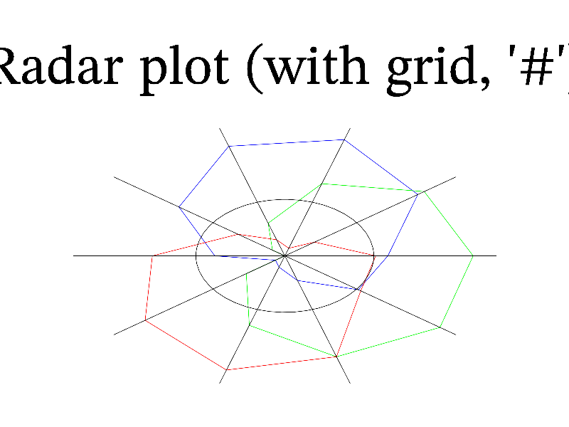
Next: region sample, Previous: radar sample, Up: All samples [Contents][Index]
Example of refill and gspline.
MGL code:
new x 10 '0.5+rnd':cumsum x 'x':norm x -1 1 copy y sin(pi*x)/1.5 subplot 2 2 0 '<_':title 'Refill sample' box:axis:plot x y 'o ':fplot 'sin(pi*x)/1.5' 'B:' new r 100:refill r x y:plot r 'r' subplot 2 2 1 '<_':title 'Global spline' box:axis:plot x y 'o ':fplot 'sin(pi*x)/1.5' 'B:' new r 100:gspline r x y:plot r 'r' new y 10 '0.5+rnd':cumsum y 'x':norm y -1 1 copy xx x:extend xx 10 copy yy y:extend yy 10:transpose yy copy z sin(pi*xx*yy)/1.5 alpha on:light on subplot 2 2 2:title '2d regular':rotate 40 60 box:axis:mesh xx yy z 'k' new rr 100 100:refill rr x y z:surf rr new xx 10 10 '(x+1)/2*cos(y*pi/2-1)':new yy 10 10 '(x+1)/2*sin(y*pi/2-1)' copy z sin(pi*xx*yy)/1.5 subplot 2 2 3:title '2d non-regular':rotate 40 60 box:axis:plot xx yy z 'ko ' new rr 100 100:refill rr xx yy z:surf rr
C++ code:
void smgl_refill(mglGraph *gr)
{
mglData x(10), y(10), r(100);
x.Modify("0.5+rnd"); x.CumSum("x"); x.Norm(-1,1);
y.Modify("sin(pi*v)/1.5",x);
if(big!=3) { gr->SubPlot(2,2,0,"<_"); gr->Title("Refill sample"); }
gr->Axis(); gr->Box(); gr->Plot(x,y,"o ");
gr->Refill(r,x,y); // or you can use r.Refill(x,y,-1,1);
gr->Plot(r,"r"); gr->FPlot("sin(pi*x)/1.5","B:");
if(big==3) return;
gr->SubPlot(2,2,1,"<_"); gr->Title("Global spline");
gr->Axis(); gr->Box(); gr->Plot(x,y,"o ");
r.RefillGS(x,y,-1,1); gr->Plot(r,"r");
gr->FPlot("sin(pi*x)/1.5","B:");
gr->Alpha(true); gr->Light(true);
mglData z(10,10), xx(10,10), yy(10,10), rr(100,100);
y.Modify("0.5+rnd"); y.CumSum("x"); y.Norm(-1,1);
for(int i=0;i<10;i++) for(int j=0;j<10;j++)
z.a[i+10*j] = sin(M_PI*x.a[i]*y.a[j])/1.5;
gr->SubPlot(2,2,2); gr->Title("2d regular"); gr->Rotate(40,60);
gr->Axis(); gr->Box(); gr->Mesh(x,y,z,"k");
gr->Refill(rr,x,y,z); gr->Surf(rr);
gr->Fill(xx,"(x+1)/2*cos(y*pi/2-1)");
gr->Fill(yy,"(x+1)/2*sin(y*pi/2-1)");
for(int i=0;i<10*10;i++)
z.a[i] = sin(M_PI*xx.a[i]*yy.a[i])/1.5;
gr->SubPlot(2,2,3); gr->Title("2d non-regular"); gr->Rotate(40,60);
gr->Axis(); gr->Box(); gr->Plot(xx,yy,z,"ko ");
gr->Refill(rr,xx,yy,z); gr->Surf(rr);
}
Next: scanfile sample, Previous: refill sample, Up: All samples [Contents][Index]
Function region fill the area between 2 curves. It support gradient filling if 2 colors per curve is specified. Also it can fill only the region y1<y<y2 if style ‘i’ is used.
MGL code:
call 'prepare1d' copy y1 y(:,1):copy y2 y(:,2) subplot 2 2 0 '':title 'Region plot (default)':box:region y1 y2:plot y1 'k2':plot y2 'k2' subplot 2 2 1 '':title '2 colors':box:region y1 y2 'yr':plot y1 'k2':plot y2 'k2' subplot 2 2 2 '':title '"i" style':box:region y1 y2 'ir':plot y1 'k2':plot y2 'k2' subplot 2 2 3 '^_':title '3d variant':rotate 40 60:box new x1 100 'sin(pi*x)':new y1 100 'cos(pi*x)':new z 100 'x' new x2 100 'sin(pi*x+pi/3)':new y2 100 'cos(pi*x+pi/3)' plot x1 y1 z 'r2':plot x2 y2 z 'b2' region x1 y1 z x2 y2 z 'cmy!'
C++ code:
void smgl_region(mglGraph *gr)
{
mglData y; mgls_prepare1d(&y);
mglData y1 = y.SubData(-1,1), y2 = y.SubData(-1,2); gr->SetOrigin(0,0,0);
if(big!=3) { gr->SubPlot(2,2,0,""); gr->Title("Region plot (default)"); }
gr->Box(); gr->Region(y1,y2); gr->Plot(y1,"k2"); gr->Plot(y2,"k2");
if(big==3) return;
gr->SubPlot(2,2,1,""); gr->Title("2 colors"); gr->Box(); gr->Region(y1,y2,"yr"); gr->Plot(y1,"k2"); gr->Plot(y2,"k2");
gr->SubPlot(2,2,2,""); gr->Title("'i' style"); gr->Box(); gr->Region(y1,y2,"ir"); gr->Plot(y1,"k2"); gr->Plot(y2,"k2");
gr->SubPlot(2,2,3,"^_"); gr->Title("3d variant"); gr->Rotate(40,60); gr->Box();
gr->Fill(y1,"cos(pi*x)"); gr->Fill(y2,"cos(pi*x+pi/3)");
mglData x1(y1.nx), x2(y1.nx), z(y1.nx);
gr->Fill(x1,"sin(pi*x)"); gr->Fill(x2,"sin(pi*x+pi/3)"); gr->Fill(z,"x");
gr->Plot(x1,y1,z,"r2"); gr->Plot(x2,y2,z,"b2");
gr->Region(x1,y1,z,x2,y2,z,"cmy!");
}
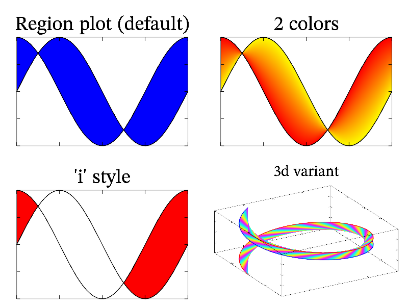
Next: schemes sample, Previous: region sample, Up: All samples [Contents][Index]
Example of scanfile for reading ’named’ data.
MGL code:
subplot 1 1 0 '<_':title 'Save and scanfile sample' list a 1 -1 0 save 'This is test: 0 -> ',a(0),' q' 'test.txt' 'w' save 'This is test: 1 -> ',a(1),' q' 'test.txt' save 'This is test: 2 -> ',a(2),' q' 'test.txt' scanfile a 'test.txt' 'This is test: %g -> %g' ranges a(0) a(1):axis:plot a(0) a(1) 'o'
C++ code:
void smgl_scanfile(mglGraph *gr)
{
gr->SubPlot(1,1,0,"<_");
if(big!=3) gr->Title("Save and scanfile sample");
FILE *fp=fopen("test.txt","w");
fprintf(fp,"This is test: 0 -> 1 q\n");
fprintf(fp,"This is test: 1 -> -1 q\n");
fprintf(fp,"This is test: 2 -> 0 q\n");
fclose(fp);
mglData a;
a.ScanFile("test.txt","This is test: %g -> %g");
gr->SetRanges(a.SubData(0), a.SubData(1));
gr->Axis(); gr->Plot(a.SubData(0),a.SubData(1),"o");
}
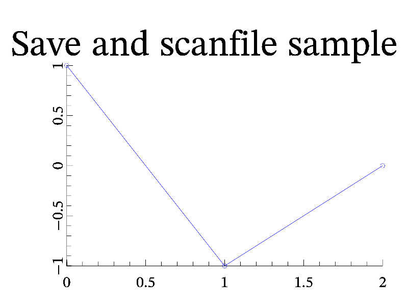
Next: section sample, Previous: scanfile sample, Up: All samples [Contents][Index]
Example of popular color schemes.
MGL code:
new x 100 100 'x':new y 100 100 'y'
call 'sch' 0 'kw'
call 'sch' 1 '%gbrw'
call 'sch' 2 'kHCcw'
call 'sch' 3 'kBbcw'
call 'sch' 4 'kRryw'
call 'sch' 5 'kGgew'
call 'sch' 6 'BbwrR'
call 'sch' 7 'BbwgG'
call 'sch' 8 'GgwmM'
call 'sch' 9 'UuwqR'
call 'sch' 10 'QqwcC'
call 'sch' 11 'CcwyY'
call 'sch' 12 'bcwyr'
call 'sch' 13 'bwr'
call 'sch' 14 'wUrqy'
call 'sch' 15 'UbcyqR'
call 'sch' 16 'BbcyrR'
call 'sch' 17 'bgr'
call 'sch' 18 'BbcyrR|'
call 'sch' 19 'b{g,0.3}r'
stop
func 'sch' 2
subplot 2 10 $1 '<>_^' 0.2 0:surfa x y $2
text 0.07+0.5*mod($1,2) 0.92-0.1*int($1/2) $2 'A'
return
C++ code:
void smgl_schemes(mglGraph *gr) // Color table
{
mglData a(256,2), b(256,2); a.Fill(-1,1); b.Fill(-1,1,'y');
gr->SubPlot(2,10,0,NULL,0.2); gr->Dens(a,"kw"); gr->Puts(0.07, 0.92, "kw", "A");
gr->SubPlot(2,10,1,NULL,0.2); gr->SurfA(a,b,"%gbrw"); gr->Puts(0.57, 0.92, "%gbrw", "A");
gr->SubPlot(2,10,2,NULL,0.2); gr->Dens(a,"kHCcw"); gr->Puts(0.07, 0.82, "kHCcw", "A");
gr->SubPlot(2,10,3,NULL,0.2); gr->Dens(a,"kBbcw"); gr->Puts(0.57, 0.82, "kBbcw", "A");
gr->SubPlot(2,10,4,NULL,0.2); gr->Dens(a,"kRryw"); gr->Puts(0.07, 0.72, "kRryw", "A");
gr->SubPlot(2,10,5,NULL,0.2); gr->Dens(a,"kGgew"); gr->Puts(0.57, 0.72, "kGgew", "A");
gr->SubPlot(2,10,6,NULL,0.2); gr->Dens(a,"BbwrR"); gr->Puts(0.07, 0.62, "BbwrR", "A");
gr->SubPlot(2,10,7,NULL,0.2); gr->Dens(a,"BbwgG"); gr->Puts(0.57, 0.62, "BbwgG", "A");
gr->SubPlot(2,10,8,NULL,0.2); gr->Dens(a,"GgwmM"); gr->Puts(0.07, 0.52, "GgwmM", "A");
gr->SubPlot(2,10,9,NULL,0.2); gr->Dens(a,"UuwqR"); gr->Puts(0.57, 0.52, "UuwqR", "A");
gr->SubPlot(2,10,10,NULL,0.2); gr->Dens(a,"QqwcC"); gr->Puts(0.07, 0.42, "QqwcC", "A");
gr->SubPlot(2,10,11,NULL,0.2); gr->Dens(a,"CcwyY"); gr->Puts(0.57, 0.42, "CcwyY", "A");
gr->SubPlot(2,10,12,NULL,0.2); gr->Dens(a,"bcwyr"); gr->Puts(0.07, 0.32, "bcwyr", "A");
gr->SubPlot(2,10,13,NULL,0.2); gr->Dens(a,"bwr"); gr->Puts(0.57, 0.32, "bwr", "A");
gr->SubPlot(2,10,14,NULL,0.2); gr->Dens(a,"wUrqy"); gr->Puts(0.07, 0.22, "wUrqy", "A");
gr->SubPlot(2,10,15,NULL,0.2); gr->Dens(a,"UbcyqR"); gr->Puts(0.57, 0.22, "UbcyqR", "A");
gr->SubPlot(2,10,16,NULL,0.2); gr->Dens(a,"BbcyrR"); gr->Puts(0.07, 0.12, "BbcyrR", "A");
gr->SubPlot(2,10,17,NULL,0.2); gr->Dens(a,"bgr"); gr->Puts(0.57, 0.12, "bgr", "A");
gr->SubPlot(2,10,18,NULL,0.2); gr->Dens(a,"BbcyrR|"); gr->Puts(0.07, 0.02, "BbcyrR|", "A");
gr->SubPlot(2,10,19,NULL,0.2); gr->Dens(a,"b{g,0.3}r"); gr->Puts(0.57, 0.02, "b\\{g,0.3\\}r", "A");
}
Next: several_light sample, Previous: schemes sample, Up: All samples [Contents][Index]
Example of section to separate data and join it back.
MGL code:
subplot 1 1 0 '<_':title 'Section&Join sample' axis:box:line -1 0 1 0 'h:' # first lets demonstrate 'join' new aa 11 'x^2':new a1 3 '-x':new a2 15 'x^3' join aa a1:join aa a2 # add x-coordinate new xx aa.nx 'x':join aa xx plot aa(:,1) aa(:,0) '2y' # now select 1-st (id=0) section between zeros section b1 aa 0 'x' 0 plot b1(:,1) b1(:,0) 'bo' # next, select 3-d (id=2) section between zeros section b3 aa 2 'x' 0 plot b3(:,1) b3(:,0) 'gs' # finally, select 2-nd (id=-2) section from the end section b4 aa -2 'x' 0 plot b4(:,1) b4(:,0) 'r#o'
C++ code:
void smgl_section(mglGraph *gr)
{
gr->SubPlot(1,1,0,"<_");
if(big!=3) gr->Title("Section&Join sample");
gr->Axis(); gr->Box(); gr->Line(mglPoint(-1,0),mglPoint(1,0),"h:");
// first lets demonstrate 'join'
mglData aa(11), a1(3), a2(15);
gr->Fill(aa,"x^2"); gr->Fill(a1,"-x"); gr->Fill(a2,"x^3");
aa.Join(a1); aa.Join(a2);
// add x-coordinate
mglData xx(aa.nx); gr->Fill(xx,"x"); aa.Join(xx);
gr->Plot(aa.SubData(-1,1), aa.SubData(-1,0), "2y");
// now select 1-st (id=0) section between zeros
mglData b1(aa.Section(0,'x',0));
gr->Plot(b1.SubData(-1,1), b1.SubData(-1,0), "bo");
// next, select 3-d (id=2) section between zeros
mglData b2(aa.Section(2,'x',0));
gr->Plot(b2.SubData(-1,1), b2.SubData(-1,0), "gs");
// finally, select 2-nd (id=-2) section from the end
mglData b3(aa.Section(-2,'x',0));
gr->Plot(b3.SubData(-1,1), b3.SubData(-1,0), "r#o");
}
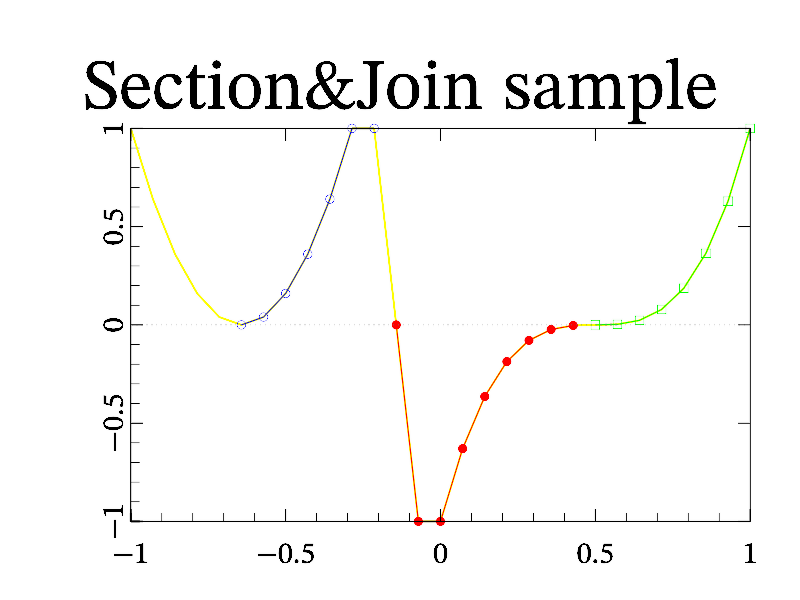
Next: solve sample, Previous: section sample, Up: All samples [Contents][Index]
Example of using several light sources.
MGL code:
call 'prepare2d' title 'Several light sources':rotate 50 60:light on light 1 0 1 0 'c':light 2 1 0 0 'y':light 3 0 -1 0 'm' box:surf a 'h'
C++ code:
void smgl_several_light(mglGraph *gr) // several light sources
{
mglData a; mgls_prepare2d(&a);
if(big!=3) gr->Title("Several light sources");
gr->Rotate(50,60); gr->Light(true); gr->AddLight(1,mglPoint(0,1,0),'c');
gr->AddLight(2,mglPoint(1,0,0),'y'); gr->AddLight(3,mglPoint(0,-1,0),'m');
gr->Box(); gr->Surf(a,"h");
}
Next: stem sample, Previous: several_light sample, Up: All samples [Contents][Index]
Example of solve for root finding.
MGL code:
zrange 0 1 new x 20 30 '(x+2)/3*cos(pi*y)' new y 20 30 '(x+2)/3*sin(pi*y)' new z 20 30 'exp(-6*x^2-2*sin(pi*y)^2)' subplot 2 1 0:title 'Cartesian space':rotate 30 -40 axis 'xyzU':box xlabel 'x':ylabel 'y' origin 1 1:grid 'xy' mesh x y z # section along 'x' direction solve u x 0.5 'x' var v u.nx 0 1 evaluate yy y u v evaluate xx x u v evaluate zz z u v plot xx yy zz 'k2o' # 1st section along 'y' direction solve u1 x -0.5 'y' var v1 u1.nx 0 1 evaluate yy y v1 u1 evaluate xx x v1 u1 evaluate zz z v1 u1 plot xx yy zz 'b2^' # 2nd section along 'y' direction solve u2 x -0.5 'y' u1 evaluate yy y v1 u2 evaluate xx x v1 u2 evaluate zz z v1 u2 plot xx yy zz 'r2v' subplot 2 1 1:title 'Accompanied space' ranges 0 1 0 1:origin 0 0 axis:box:xlabel 'i':ylabel 'j':grid2 z 'h' plot u v 'k2o':line 0.4 0.5 0.8 0.5 'kA' plot v1 u1 'b2^':line 0.5 0.15 0.5 0.3 'bA' plot v1 u2 'r2v':line 0.5 0.7 0.5 0.85 'rA'
C++ code:
void smgl_solve(mglGraph *gr) // solve and evaluate
{
gr->SetRange('z',0,1);
mglData x(20,30), y(20,30), z(20,30), xx,yy,zz;
gr->Fill(x,"(x+2)/3*cos(pi*y)");
gr->Fill(y,"(x+2)/3*sin(pi*y)");
gr->Fill(z,"exp(-6*x^2-2*sin(pi*y)^2)");
gr->SubPlot(2,1,0); gr->Title("Cartesian space"); gr->Rotate(30,-40);
gr->Axis("xyzU"); gr->Box(); gr->Label('x',"x"); gr->Label('y',"y");
gr->SetOrigin(1,1); gr->Grid("xy");
gr->Mesh(x,y,z);
// section along 'x' direction
mglData u = x.Solve(0.5,'x');
mglData v(u.nx); v.Fill(0,1);
xx = x.Evaluate(u,v); yy = y.Evaluate(u,v); zz = z.Evaluate(u,v);
gr->Plot(xx,yy,zz,"k2o");
// 1st section along 'y' direction
mglData u1 = x.Solve(-0.5,'y');
mglData v1(u1.nx); v1.Fill(0,1);
xx = x.Evaluate(v1,u1); yy = y.Evaluate(v1,u1); zz = z.Evaluate(v1,u1);
gr->Plot(xx,yy,zz,"b2^");
// 2nd section along 'y' direction
mglData u2 = x.Solve(-0.5,'y',u1);
xx = x.Evaluate(v1,u2); yy = y.Evaluate(v1,u2); zz = z.Evaluate(v1,u2);
gr->Plot(xx,yy,zz,"r2v");
gr->SubPlot(2,1,1); gr->Title("Accompanied space");
gr->SetRanges(0,1,0,1); gr->SetOrigin(0,0);
gr->Axis(); gr->Box(); gr->Label('x',"i"); gr->Label('y',"j");
gr->Grid(z,"h");
gr->Plot(u,v,"k2o"); gr->Line(mglPoint(0.4,0.5),mglPoint(0.8,0.5),"kA");
gr->Plot(v1,u1,"b2^"); gr->Line(mglPoint(0.5,0.15),mglPoint(0.5,0.3),"bA");
gr->Plot(v1,u2,"r2v"); gr->Line(mglPoint(0.5,0.7),mglPoint(0.5,0.85),"rA");
}
Next: step sample, Previous: solve sample, Up: All samples [Contents][Index]
Function stem draw vertical bars. It is most attractive if markers are drawn too.
MGL code:
call 'prepare1d' origin 0 0 0:subplot 2 2 0 '':title 'Stem plot (default)':box:stem y new yc 30 'sin(pi*x)':new xc 30 'cos(pi*x)':new z 30 'x' subplot 2 2 1:title '3d variant':rotate 50 60:box:stem xc yc z 'rx' subplot 2 2 2 '':title '"!" style':box:stem y 'o!rgb'
C++ code:
void smgl_stem(mglGraph *gr)
{
mglData y; mgls_prepare1d(&y); gr->SetOrigin(0,0,0);
mglData yc(30), xc(30), z(30); z.Modify("2*x-1");
yc.Modify("sin(pi*(2*x-1))"); xc.Modify("cos(pi*2*x-pi)");
if(big!=3) { gr->SubPlot(2,2,0,""); gr->Title("Stem plot (default)"); }
gr->Box(); gr->Stem(y);
if(big==3) return;
gr->SubPlot(2,2,1); gr->Title("3d variant"); gr->Rotate(50,60);
gr->Box(); gr->Stem(xc,yc,z,"rx");
gr->SubPlot(2,2,2,""); gr->Title("'!' style"); gr->Box(); gr->Stem(y,"o!rgb");
}
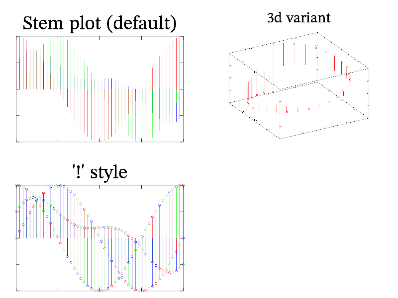
Next: stereo sample, Previous: stem sample, Up: All samples [Contents][Index]
Function step plot data as stairs. At this stairs can be centered if sizes are differ by 1.
MGL code:
call 'prepare1d' origin 0 0 0:subplot 2 2 0 '':title 'Step plot (default)':box:step y new yc 30 'sin(pi*x)':new xc 30 'cos(pi*x)':new z 30 'x' subplot 2 2 1:title '3d variant':rotate 50 60:box:step xc yc z 'r' subplot 2 2 2 '':title '"!" style':box:step y 's!rgb'
C++ code:
void smgl_step(mglGraph *gr)
{
mglData y; mgls_prepare1d(&y); gr->SetOrigin(0,0,0);
mglData yc(30), xc(30), z(30); z.Modify("2*x-1");
yc.Modify("sin(pi*(2*x-1))"); xc.Modify("cos(pi*2*x-pi)");
if(big!=3) { gr->SubPlot(2,2,0,""); gr->Title("Step plot (default)"); }
gr->Box(); gr->Step(y);
if(big==3) return;
gr->SubPlot(2,2,1); gr->Title("3d variant"); gr->Rotate(50,60);
gr->Box(); gr->Step(xc,yc,z,"r");
gr->SubPlot(2,2,2,""); gr->Title("'!' style"); gr->Box(); gr->Step(y,"s!rgb");
}
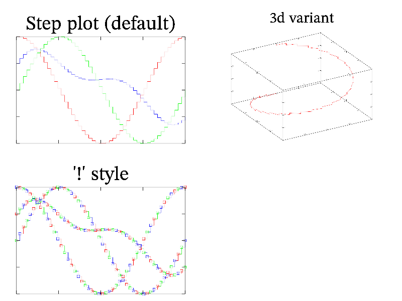
Next: stfa sample, Previous: step sample, Up: All samples [Contents][Index]
Example of stereo image of surf.
MGL code:
call 'prepare2d' light on subplot 2 1 0:rotate 50 60+1:box:surf a subplot 2 1 1:rotate 50 60-1:box:surf a
C++ code:
void smgl_stereo(mglGraph *gr)
{
mglData a; mgls_prepare2d(&a);
gr->Light(true);
gr->SubPlot(2,1,0); gr->Rotate(50,60+1);
gr->Box(); gr->Surf(a);
gr->SubPlot(2,1,1); gr->Rotate(50,60-1);
gr->Box(); gr->Surf(a);
}
Next: style sample, Previous: stereo sample, Up: All samples [Contents][Index]
Example of stfa.
MGL code:
new a 2000:new b 2000 fill a 'cos(50*pi*x)*(x<-.5)+cos(100*pi*x)*(x<0)*(x>-.5)+\ cos(200*pi*x)*(x<.5)*(x>0)+cos(400*pi*x)*(x>.5)' subplot 1 2 0 '<_':title 'Initial signal':plot a:axis:xlabel '\i t' subplot 1 2 1 '<_':title 'STFA plot':stfa a b 64:axis:ylabel '\omega' 0:xlabel '\i t'
C++ code:
void smgl_stfa(mglGraph *gr) // STFA sample
{
mglData a(2000), b(2000);
gr->Fill(a,"cos(50*pi*x)*(x<-.5)+cos(100*pi*x)*(x<0)*(x>-.5)+\
cos(200*pi*x)*(x<.5)*(x>0)+cos(400*pi*x)*(x>.5)");
gr->SubPlot(1, 2, 0,"<_"); gr->Title("Initial signal");
gr->Plot(a);
gr->Axis();
gr->Label('x', "\\i t");
gr->SubPlot(1, 2, 1,"<_"); gr->Title("STFA plot");
gr->STFA(a, b, 64);
gr->Axis();
gr->Label('x', "\\i t");
gr->Label('y', "\\omega", 0);
}
Next: surf sample, Previous: stfa sample, Up: All samples [Contents][Index]
Example of colors and styles for plots.
MGL code:
C++ code:
void smgl_style(mglGraph *gr) // pen styles
{
gr->SubPlot(2,2,0);
double d,x1,x2,x0,y=1.1, y1=1.15;
d=0.3, x0=0.2, x1=0.5, x2=0.6;
gr->Line(mglPoint(x0,y1-0*d),mglPoint(x1,y1-0*d),"k-"); gr->Puts(mglPoint(x2,y-0*d),"Solid '-'",":rL");
gr->Line(mglPoint(x0,y1-1*d),mglPoint(x1,y1-1*d),"k|"); gr->Puts(mglPoint(x2,y-1*d),"Long Dash '|'",":rL");
gr->Line(mglPoint(x0,y1-2*d),mglPoint(x1,y1-2*d),"k;"); gr->Puts(mglPoint(x2,y-2*d),"Dash ';'",":rL");
gr->Line(mglPoint(x0,y1-3*d),mglPoint(x1,y1-3*d),"k="); gr->Puts(mglPoint(x2,y-3*d),"Small dash '='",":rL");
gr->Line(mglPoint(x0,y1-4*d),mglPoint(x1,y1-4*d),"kj"); gr->Puts(mglPoint(x2,y-4*d),"Dash-dot 'j'",":rL");
gr->Line(mglPoint(x0,y1-5*d),mglPoint(x1,y1-5*d),"ki"); gr->Puts(mglPoint(x2,y-5*d),"Small dash-dot 'i'",":rL");
gr->Line(mglPoint(x0,y1-6*d),mglPoint(x1,y1-6*d),"k:"); gr->Puts(mglPoint(x2,y-6*d),"Dots ':'",":rL");
gr->Line(mglPoint(x0,y1-7*d),mglPoint(x1,y1-7*d),"k "); gr->Puts(mglPoint(x2,y-7*d),"None ' '",":rL");
gr->Line(mglPoint(x0,y1-8*d),mglPoint(x1,y1-8*d),"k{df090}"); gr->Puts(mglPoint(x2,y-8*d),"Manual '{df090}'",":rL");
d=0.25; x1=-1; x0=-0.8; y = -0.05;
gr->Mark(mglPoint(x1,5*d),"k."); gr->Puts(mglPoint(x0,y+5*d),"'.'",":rL");
gr->Mark(mglPoint(x1,4*d),"k+"); gr->Puts(mglPoint(x0,y+4*d),"'+'",":rL");
gr->Mark(mglPoint(x1,3*d),"kx"); gr->Puts(mglPoint(x0,y+3*d),"'x'",":rL");
gr->Mark(mglPoint(x1,2*d),"k*"); gr->Puts(mglPoint(x0,y+2*d),"'*'",":rL");
gr->Mark(mglPoint(x1,d),"ks"); gr->Puts(mglPoint(x0,y+d),"'s'",":rL");
gr->Mark(mglPoint(x1,0),"kd"); gr->Puts(mglPoint(x0,y),"'d'",":rL");
gr->Mark(mglPoint(x1,-d,0),"ko"); gr->Puts(mglPoint(x0,y-d),"'o'",":rL");
gr->Mark(mglPoint(x1,-2*d,0),"k^"); gr->Puts(mglPoint(x0,y-2*d),"'\\^'",":rL");
gr->Mark(mglPoint(x1,-3*d,0),"kv"); gr->Puts(mglPoint(x0,y-3*d),"'v'",":rL");
gr->Mark(mglPoint(x1,-4*d,0),"k<"); gr->Puts(mglPoint(x0,y-4*d),"'<'",":rL");
gr->Mark(mglPoint(x1,-5*d,0),"k>"); gr->Puts(mglPoint(x0,y-5*d),"'>'",":rL");
d=0.25; x1=-0.5; x0=-0.3; y = -0.05;
gr->Mark(mglPoint(x1,5*d),"k#."); gr->Puts(mglPoint(x0,y+5*d),"'\\#.'",":rL");
gr->Mark(mglPoint(x1,4*d),"k#+"); gr->Puts(mglPoint(x0,y+4*d),"'\\#+'",":rL");
gr->Mark(mglPoint(x1,3*d),"k#x"); gr->Puts(mglPoint(x0,y+3*d),"'\\#x'",":rL");
gr->Mark(mglPoint(x1,2*d),"k#*"); gr->Puts(mglPoint(x0,y+2*d),"'\\#*'",":rL");
gr->Mark(mglPoint(x1,d),"k#s"); gr->Puts(mglPoint(x0,y+d),"'\\#s'",":rL");
gr->Mark(mglPoint(x1,0),"k#d"); gr->Puts(mglPoint(x0,y),"'\\#d'",":rL");
gr->Mark(mglPoint(x1,-d,0),"k#o"); gr->Puts(mglPoint(x0,y-d),"'\\#o'",":rL");
gr->Mark(mglPoint(x1,-2*d,0),"k#^"); gr->Puts(mglPoint(x0,y-2*d),"'\\#\\^'",":rL");
gr->Mark(mglPoint(x1,-3*d,0),"k#v"); gr->Puts(mglPoint(x0,y-3*d),"'\\#v'",":rL");
gr->Mark(mglPoint(x1,-4*d,0),"k#<"); gr->Puts(mglPoint(x0,y-4*d),"'\\#<'",":rL");
gr->Mark(mglPoint(x1,-5*d,0),"k#>"); gr->Puts(mglPoint(x0,y-5*d),"'\\#>'",":rL");
gr->SubPlot(2,2,1);
double a=0.1,b=0.4,c=0.5;
gr->Line(mglPoint(a,1),mglPoint(b,1),"k-A"); gr->Puts(mglPoint(c,1),"Style 'A' or 'A\\_'",":rL");
gr->Line(mglPoint(a,0.8),mglPoint(b,0.8),"k-V"); gr->Puts(mglPoint(c,0.8),"Style 'V' or 'V\\_'",":rL");
gr->Line(mglPoint(a,0.6),mglPoint(b,0.6),"k-K"); gr->Puts(mglPoint(c,0.6),"Style 'K' or 'K\\_'",":rL");
gr->Line(mglPoint(a,0.4),mglPoint(b,0.4),"k-I"); gr->Puts(mglPoint(c,0.4),"Style 'I' or 'I\\_'",":rL");
gr->Line(mglPoint(a,0.2),mglPoint(b,0.2),"k-D"); gr->Puts(mglPoint(c,0.2),"Style 'D' or 'D\\_'",":rL");
gr->Line(mglPoint(a,0),mglPoint(b,0),"k-S"); gr->Puts(mglPoint(c,0),"Style 'S' or 'S\\_'",":rL");
gr->Line(mglPoint(a,-0.2),mglPoint(b,-0.2),"k-O"); gr->Puts(mglPoint(c,-0.2),"Style 'O' or 'O\\_'",":rL");
gr->Line(mglPoint(a,-0.4),mglPoint(b,-0.4),"k-T"); gr->Puts(mglPoint(c,-0.4),"Style 'T' or 'T\\_'",":rL");
gr->Line(mglPoint(a,-0.6),mglPoint(b,-0.6),"k-X"); gr->Puts(mglPoint(c,-0.6),"Style 'X' or 'X\\_'",":rL");
gr->Line(mglPoint(a,-0.8),mglPoint(b,-0.8),"k-_"); gr->Puts(mglPoint(c,-0.8),"Style '\\_' or none",":rL");
gr->Line(mglPoint(a,-1),mglPoint(b,-1),"k-AS"); gr->Puts(mglPoint(c,-1),"Style 'AS'",":rL");
gr->Line(mglPoint(a,-1.2),mglPoint(b,-1.2),"k-_A"); gr->Puts(mglPoint(c,-1.2),"Style '\\_A'",":rL");
a=-1; b=-0.7; c=-0.6;
gr->Line(mglPoint(a,1),mglPoint(b,1),"kAA"); gr->Puts(mglPoint(c,1),"Style 'AA'",":rL");
gr->Line(mglPoint(a,0.8),mglPoint(b,0.8),"kVV"); gr->Puts(mglPoint(c,0.8),"Style 'VV'",":rL");
gr->Line(mglPoint(a,0.6),mglPoint(b,0.6),"kKK"); gr->Puts(mglPoint(c,0.6),"Style 'KK'",":rL");
gr->Line(mglPoint(a,0.4),mglPoint(b,0.4),"kII"); gr->Puts(mglPoint(c,0.4),"Style 'II'",":rL");
gr->Line(mglPoint(a,0.2),mglPoint(b,0.2),"kDD"); gr->Puts(mglPoint(c,0.2),"Style 'DD'",":rL");
gr->Line(mglPoint(a,0),mglPoint(b,0),"kSS"); gr->Puts(mglPoint(c,0),"Style 'SS'",":rL");
gr->Line(mglPoint(a,-0.2),mglPoint(b,-0.2),"kOO"); gr->Puts(mglPoint(c,-0.2),"Style 'OO'",":rL");
gr->Line(mglPoint(a,-0.4),mglPoint(b,-0.4),"kTT"); gr->Puts(mglPoint(c,-0.4),"Style 'TT'",":rL");
gr->Line(mglPoint(a,-0.6),mglPoint(b,-0.6),"kXX"); gr->Puts(mglPoint(c,-0.6),"Style 'XX'",":rL");
gr->Line(mglPoint(a,-0.8),mglPoint(b,-0.8),"k-__"); gr->Puts(mglPoint(c,-0.8),"Style '\\_\\_'",":rL");
gr->Line(mglPoint(a,-1),mglPoint(b,-1),"k-VA"); gr->Puts(mglPoint(c,-1),"Style 'VA'",":rL");
gr->Line(mglPoint(a,-1.2),mglPoint(b,-1.2),"k-AV"); gr->Puts(mglPoint(c,-1.2),"Style 'AV'",":rL");
gr->SubPlot(2,2,2);
//#LENUQ
gr->FaceZ(mglPoint(-1, -1), 0.4, 0.3, "L#"); gr->Puts(mglPoint(-0.8,-0.9), "L", "w:C", -1.4);
gr->FaceZ(mglPoint(-0.6,-1), 0.4, 0.3, "E#"); gr->Puts(mglPoint(-0.4,-0.9), "E", "w:C", -1.4);
gr->FaceZ(mglPoint(-0.2,-1), 0.4, 0.3, "N#"); gr->Puts(mglPoint(0, -0.9), "N", "w:C", -1.4);
gr->FaceZ(mglPoint(0.2, -1), 0.4, 0.3, "U#"); gr->Puts(mglPoint(0.4,-0.9), "U", "w:C", -1.4);
gr->FaceZ(mglPoint(0.6, -1), 0.4, 0.3, "Q#"); gr->Puts(mglPoint(0.8,-0.9), "Q", "w:C", -1.4);
//#lenuq
gr->FaceZ(mglPoint(-1, -0.7), 0.4, 0.3, "l#"); gr->Puts(mglPoint(-0.8,-0.6), "l", "k:C", -1.4);
gr->FaceZ(mglPoint(-0.6,-0.7), 0.4, 0.3, "e#"); gr->Puts(mglPoint(-0.4,-0.6), "e", "k:C", -1.4);
gr->FaceZ(mglPoint(-0.2,-0.7), 0.4, 0.3, "n#"); gr->Puts(mglPoint(0, -0.6), "n", "k:C", -1.4);
gr->FaceZ(mglPoint(0.2, -0.7), 0.4, 0.3, "u#"); gr->Puts(mglPoint(0.4,-0.6), "u", "k:C", -1.4);
gr->FaceZ(mglPoint(0.6, -0.7), 0.4, 0.3, "q#"); gr->Puts(mglPoint(0.8,-0.6), "q", "k:C", -1.4);
//#CMYkP
gr->FaceZ(mglPoint(-1, -0.4), 0.4, 0.3, "C#"); gr->Puts(mglPoint(-0.8,-0.3), "C", "w:C", -1.4);
gr->FaceZ(mglPoint(-0.6,-0.4), 0.4, 0.3, "M#"); gr->Puts(mglPoint(-0.4,-0.3), "M", "w:C", -1.4);
gr->FaceZ(mglPoint(-0.2,-0.4), 0.4, 0.3, "Y#"); gr->Puts(mglPoint(0, -0.3), "Y", "w:C", -1.4);
gr->FaceZ(mglPoint(0.2, -0.4), 0.4, 0.3, "k#"); gr->Puts(mglPoint(0.4,-0.3), "k", "w:C", -1.4);
gr->FaceZ(mglPoint(0.6, -0.4), 0.4, 0.3, "P#"); gr->Puts(mglPoint(0.8,-0.3), "P", "w:C", -1.4);
//#cmywp
gr->FaceZ(mglPoint(-1, -0.1), 0.4, 0.3, "c#"); gr->Puts(mglPoint(-0.8, 0), "c", "k:C", -1.4);
gr->FaceZ(mglPoint(-0.6,-0.1), 0.4, 0.3, "m#"); gr->Puts(mglPoint(-0.4, 0), "m", "k:C", -1.4);
gr->FaceZ(mglPoint(-0.2,-0.1), 0.4, 0.3, "y#"); gr->Puts(mglPoint(0, 0), "y", "k:C", -1.4);
gr->FaceZ(mglPoint(0.2, -0.1), 0.4, 0.3, "w#"); gr->Puts(mglPoint(0.4, 0), "w", "k:C", -1.4);
gr->FaceZ(mglPoint(0.6, -0.1), 0.4, 0.3, "p#"); gr->Puts(mglPoint(0.8, 0), "p", "k:C", -1.4);
//#BGRHW
gr->FaceZ(mglPoint(-1, 0.2), 0.4, 0.3, "B#"); gr->Puts(mglPoint(-0.8, 0.3), "B", "w:C", -1.4);
gr->FaceZ(mglPoint(-0.6,0.2), 0.4, 0.3, "G#"); gr->Puts(mglPoint(-0.4, 0.3), "G", "w:C", -1.4);
gr->FaceZ(mglPoint(-0.2,0.2), 0.4, 0.3, "R#"); gr->Puts(mglPoint(0, 0.3), "R", "w:C", -1.4);
gr->FaceZ(mglPoint(0.2, 0.2), 0.4, 0.3, "H#"); gr->Puts(mglPoint(0.4, 0.3), "H", "w:C", -1.4);
gr->FaceZ(mglPoint(0.6, 0.2), 0.4, 0.3, "W#"); gr->Puts(mglPoint(0.8, 0.3), "W", "w:C", -1.4);
//#bgrhw
gr->FaceZ(mglPoint(-1, 0.5), 0.4, 0.3, "b#"); gr->Puts(mglPoint(-0.8, 0.6), "b", "k:C", -1.4);
gr->FaceZ(mglPoint(-0.6,0.5), 0.4, 0.3, "g#"); gr->Puts(mglPoint(-0.4, 0.6), "g", "k:C", -1.4);
gr->FaceZ(mglPoint(-0.2,0.5), 0.4, 0.3, "r#"); gr->Puts(mglPoint(0, 0.6), "r", "k:C", -1.4);
gr->FaceZ(mglPoint(0.2, 0.5), 0.4, 0.3, "h#"); gr->Puts(mglPoint(0.4, 0.6), "h", "k:C", -1.4);
gr->FaceZ(mglPoint(0.6, 0.5), 0.4, 0.3, "w#"); gr->Puts(mglPoint(0.8, 0.6), "w", "k:C", -1.4);
//#brighted
gr->FaceZ(mglPoint(-1, 0.8), 0.4, 0.3, "{r1}#"); gr->Puts(mglPoint(-0.8, 0.9), "\\{r1\\}", "w:C", -1.4);
gr->FaceZ(mglPoint(-0.6,0.8), 0.4, 0.3, "{r3}#"); gr->Puts(mglPoint(-0.4, 0.9), "\\{r3\\}", "w:C", -1.4);
gr->FaceZ(mglPoint(-0.2,0.8), 0.4, 0.3, "{r5}#"); gr->Puts(mglPoint(0, 0.9), "\\{r5\\}", "k:C", -1.4);
gr->FaceZ(mglPoint(0.2, 0.8), 0.4, 0.3, "{r7}#"); gr->Puts(mglPoint(0.4, 0.9), "\\{r7\\}", "k:C", -1.4);
gr->FaceZ(mglPoint(0.6, 0.8), 0.4, 0.3, "{r9}#"); gr->Puts(mglPoint(0.8, 0.9), "\\{r9\\}", "k:C", -1.4);
// HEX
gr->FaceZ(mglPoint(-1, -1.3), 1, 0.3, "{xff9966}#"); gr->Puts(mglPoint(-0.5,-1.2), "\\{xff9966\\}", "k:C", -1.4);
gr->FaceZ(mglPoint(0, -1.3), 1, 0.3, "{x83CAFF}#"); gr->Puts(mglPoint( 0.5,-1.2), "\\{x83CAFF\\}", "k:C", -1.4);
gr->SubPlot(2,2,3);
char stl[3]="r1", txt[4]="'1'";
for(int i=0;i<10;i++)
{
txt[1]=stl[1]='0'+i;
gr->Line(mglPoint(-1,0.2*i-1),mglPoint(1,0.2*i-1),stl);
gr->Puts(mglPoint(1.05,0.2*i-1),txt,":L");
}
}
Next: surf3 sample, Previous: style sample, Up: All samples [Contents][Index]
Function surf is most standard way to visualize 2D data array. Surf use color scheme for coloring (see Color scheme). You can use ‘#’ style for drawing black meshes on the surface.
MGL code:
call 'prepare2d' subplot 2 2 0:title 'Surf plot (default)':rotate 50 60:light on:box:surf a subplot 2 2 1:title '"\#" style; meshnum 10':rotate 50 60:box:surf a '#'; meshnum 10 subplot 2 2 2:title '"." style':rotate 50 60:box:surf a '.' new x 50 40 '0.8*sin(pi*x)*sin(pi*(y+1)/2)' new y 50 40 '0.8*cos(pi*x)*sin(pi*(y+1)/2)' new z 50 40 '0.8*cos(pi*(y+1)/2)' subplot 2 2 3:title 'parametric form':rotate 50 60:box:surf x y z 'BbwrR'
C++ code:
void smgl_surf3(mglGraph *gr)
{
mglData c; mgls_prepare3d(&c);
if(big!=3) { gr->SubPlot(2,2,0); gr->Title("Surf3 plot (default)"); }
gr->Rotate(50,60); gr->Light(true); gr->Alpha(true);
gr->Box(); gr->Surf3(c);
if(big==3) return;
gr->SubPlot(2,2,1); gr->Title("'\\#' style");
gr->Rotate(50,60); gr->Box(); gr->Surf3(c,"#");
gr->SubPlot(2,2,2); gr->Title("'.' style");
gr->Rotate(50,60); gr->Box(); gr->Surf3(c,".");
}

Next: surf3a sample, Previous: surf sample, Up: All samples [Contents][Index]
Function surf3 is one of most suitable (for my opinion) functions to visualize 3D data. It draw the isosurface(s) – surface(s) of constant amplitude (3D analogue of contour lines). You can draw wired isosurfaces if specify ‘#’ style.
MGL code:
call 'prepare3d' light on:alpha on subplot 2 2 0:title 'Surf3 plot (default)' rotate 50 60:box:surf3 c subplot 2 2 1:title '"\#" style' rotate 50 60:box:surf3 c '#' subplot 2 2 2:title '"." style' rotate 50 60:box:surf3 c '.'
C++ code:
void smgl_surf3(mglGraph *gr)
{
mglData c; mgls_prepare3d(&c);
if(big!=3) { gr->SubPlot(2,2,0); gr->Title("Surf3 plot (default)"); }
gr->Rotate(50,60); gr->Light(true); gr->Alpha(true);
gr->Box(); gr->Surf3(c);
if(big==3) return;
gr->SubPlot(2,2,1); gr->Title("'\\#' style");
gr->Rotate(50,60); gr->Box(); gr->Surf3(c,"#");
gr->SubPlot(2,2,2); gr->Title("'.' style");
gr->Rotate(50,60); gr->Box(); gr->Surf3(c,".");
}
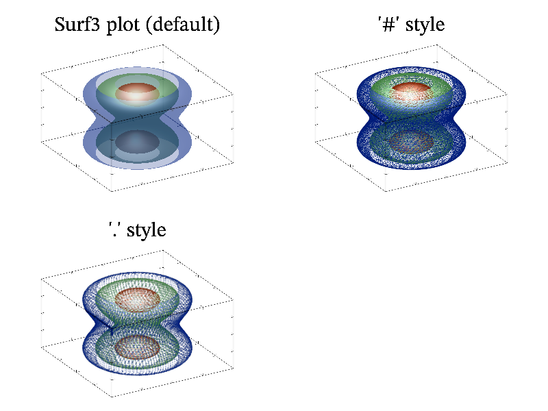
Next: surf3c sample, Previous: surf3 sample, Up: All samples [Contents][Index]
Function surf3c is similar to surf3 but its transparency is determined by another data.
MGL code:
call 'prepare3d' title 'Surf3A plot':rotate 50 60:light on:alpha on:box:surf3a c d
C++ code:
void smgl_surf3a(mglGraph *gr)
{
mglData c,d; mgls_prepare3d(&c,&d);
if(big!=3) gr->Title("Surf3A plot");
gr->Rotate(50,60); gr->Light(true); gr->Alpha(true);
gr->Box(); gr->Surf3A(c,d);
}

Next: surf3ca sample, Previous: surf3a sample, Up: All samples [Contents][Index]
Function surf3c is similar to surf3 but its coloring is determined by another data.
MGL code:
call 'prepare3d' title 'Surf3C plot':rotate 50 60:light on:alpha on:box:surf3c c d
C++ code:
void smgl_surf3c(mglGraph *gr)
{
mglData c,d; mgls_prepare3d(&c,&d);
if(big!=3) gr->Title("Surf3C plot");
gr->Rotate(50,60); gr->Light(true); gr->Alpha(true);
gr->Box(); gr->Surf3C(c,d);
}
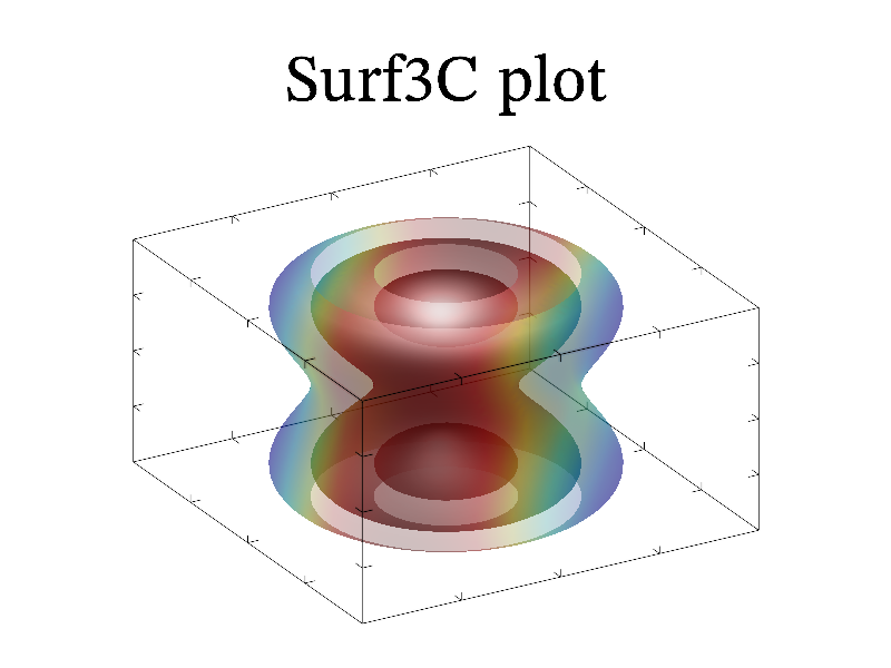
Next: surfa sample, Previous: surf3c sample, Up: All samples [Contents][Index]
Function surf3c is similar to surf3 but its coloring and transparency is determined by another data arrays.
MGL code:
call 'prepare3d' title 'Surf3CA plot':rotate 50 60:light on:alpha on:box:surf3ca c d c
C++ code:
void smgl_surf3ca(mglGraph *gr)
{
mglData c,d; mgls_prepare3d(&c,&d);
if(big!=3) gr->Title("Surf3CA plot");
gr->Rotate(50,60); gr->Light(true); gr->Alpha(true);
gr->Box(); gr->Surf3CA(c,d,c);
}
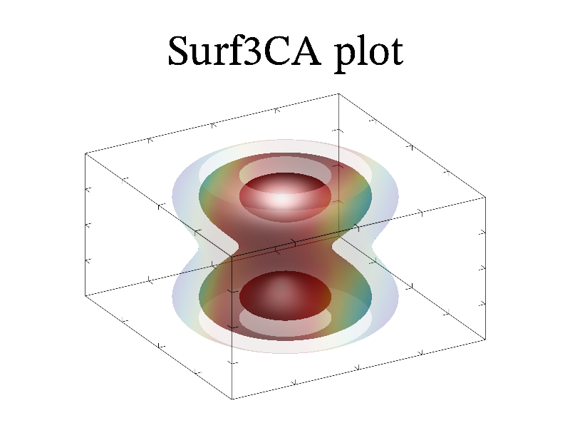
Next: surfc sample, Previous: surf3ca sample, Up: All samples [Contents][Index]
Function surfa is similar to surf but its transparency is determined by another data.
MGL code:
call 'prepare2d' title 'SurfA plot':rotate 50 60:light on:alpha on:box:surfa a b
C++ code:
void smgl_surfa(mglGraph *gr)
{
mglData a,b; mgls_prepare2d(&a,&b);
if(big!=3) gr->Title("SurfA plot");
gr->Rotate(50,60); gr->Alpha(true); gr->Light(true); gr->Box();
gr->SurfA(a,b);
}

Next: surfca sample, Previous: surfa sample, Up: All samples [Contents][Index]
Function surfc is similar to surf but its coloring is determined by another data.
MGL code:
call 'prepare2d' title 'SurfC plot':rotate 50 60:light on:box:surfc a b
C++ code:
void smgl_surfc(mglGraph *gr)
{
mglData a,b; mgls_prepare2d(&a,&b);
if(big!=3) gr->Title("SurfC plot");
gr->Rotate(50,60); gr->Light(true); gr->Box(); gr->SurfC(a,b);
}
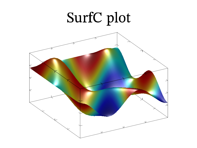
Next: table sample, Previous: surfc sample, Up: All samples [Contents][Index]
Function surfca is similar to surf but its coloring and transparency is determined by another data arrays.
MGL code:
call 'prepare2d' title 'SurfCA plot':rotate 50 60:light on:alpha on:box:surfca a b a
C++ code:
void smgl_surfca(mglGraph *gr)
{
mglData a,b; mgls_prepare2d(&a,&b);
if(big!=3) gr->Title("SurfCA plot");
gr->Rotate(50,60); gr->Alpha(true); gr->Light(true); gr->Box();
gr->SurfCA(a,b,a);
}

Next: tape sample, Previous: surfca sample, Up: All samples [Contents][Index]
Function table draw table with data values.
MGL code:
new ys 10 3 '0.8*sin(pi*(x+y/4+1.25))+0.2*rnd'
subplot 2 2 0:title 'Table sample':box
table ys 'y_1\n{}y_2\n{}y_3'
subplot 2 2 1:title 'no borders, colored'
table ys 'y_1\n{}y_2\n{}y_3' 'r|'
subplot 2 2 2:title 'no font decrease'
table ys 'y_1\n{}y_2\n{}y_3' '#'
subplot 2 2 3:title 'manual width and position':box
table 0.5 0.95 ys 'y_1\n{}y_2\n{}y_3' '#';value 0.7
C++ code:
void smgl_table(mglGraph *gr)
{
mglData ys(10,3); ys.Modify("0.8*sin(pi*(2*x+y/2))+0.2*rnd");
if(big!=3) { gr->SubPlot(2,2,0); gr->Title("Table plot"); }
gr->Table(ys,"y_1\ny_2\ny_3"); gr->Box();
if(big==3) return;
gr->SubPlot(2,2,1); gr->Title("no borders, colored");
gr->Table(ys,"y_1\ny_2\ny_3","r|");
gr->SubPlot(2,2,2); gr->Title("no font decrease");
gr->Table(ys,"y_1\ny_2\ny_3","#");
gr->SubPlot(2,2,3); gr->Title("manual width, position");
gr->Table(0.5, 0.95, ys,"y_1\ny_2\ny_3","#", "value 0.7"); gr->Box();
}

Next: tens sample, Previous: table sample, Up: All samples [Contents][Index]
Function tape draw tapes which rotate around the curve as transverse orts of accompanied coordinates.
MGL code:
call 'prepare1d' new yc 50 'sin(pi*x)':new xc 50 'cos(pi*x)':new z 50 'x' subplot 2 2 0 '':title 'Tape plot (default)':box:tape y:plot y 'k' subplot 2 2 1:title '3d variant, 2 colors':rotate 50 60:light on box:plot xc yc z 'k':tape xc yc z 'rg' subplot 2 2 2:title '3d variant, x only':rotate 50 60 box:plot xc yc z 'k':tape xc yc z 'xr':tape xc yc z 'xr#' subplot 2 2 3:title '3d variant, z only':rotate 50 60 box:plot xc yc z 'k':tape xc yc z 'zg':tape xc yc z 'zg#'
C++ code:
void smgl_tape(mglGraph *gr)
{
mglData y; mgls_prepare1d(&y);
mglData xc(50), yc(50), z(50);
yc.Modify("sin(pi*(2*x-1))");
xc.Modify("cos(pi*2*x-pi)"); z.Fill(-1,1);
if(big!=3) { gr->SubPlot(2,2,0,""); gr->Title("Tape plot (default)"); }
gr->Box(); gr->Tape(y); gr->Plot(y,"k");
if(big==3) return;
gr->SubPlot(2,2,1); gr->Title("3d variant, 2 colors"); gr->Rotate(50,60); gr->Light(true);
gr->Box(); gr->Plot(xc,yc,z,"k"); gr->Tape(xc,yc,z,"rg");
gr->SubPlot(2,2,2); gr->Title("3d variant, x only"); gr->Rotate(50,60);
gr->Box(); gr->Plot(xc,yc,z,"k"); gr->Tape(xc,yc,z,"xr"); gr->Tape(xc,yc,z,"xr#");
gr->SubPlot(2,2,3); gr->Title("3d variant, z only"); gr->Rotate(50,60);
gr->Box(); gr->Plot(xc,yc,z,"k"); gr->Tape(xc,yc,z,"zg"); gr->Tape(xc,yc,z,"zg#");
}
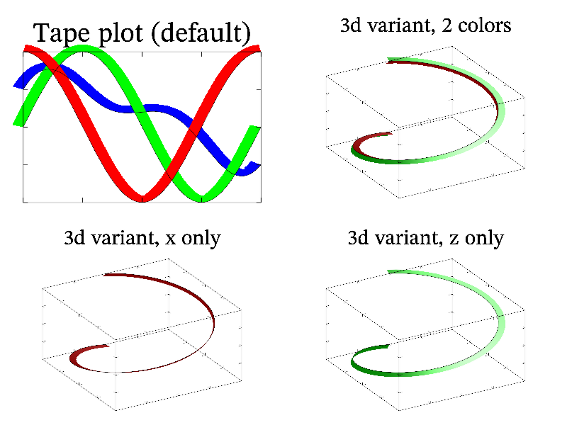
Next: ternary sample, Previous: tape sample, Up: All samples [Contents][Index]
Function tens is variant of plot with smooth coloring along the curves. At this, color is determined as for surfaces (see Color scheme).
MGL code:
call 'prepare1d' subplot 2 2 0 '':title 'Tens plot (default)':box:tens y(:,0) y(:,1) subplot 2 2 2 '':title '" " style':box:tens y(:,0) y(:,1) 'o ' new yc 30 'sin(pi*x)':new xc 30 'cos(pi*x)':new z 30 'x' subplot 2 2 1:title '3d variant':rotate 50 60:box:tens xc yc z z 's'
C++ code:
void smgl_tens(mglGraph *gr)
{
mglData y; mgls_prepare1d(&y); gr->SetOrigin(0,0,0);
if(big!=3) { gr->SubPlot(2,2,0,""); gr->Title("Tens plot (default)"); }
gr->Box(); gr->Tens(y.SubData(-1,0), y.SubData(-1,1));
if(big==3) return;
gr->SubPlot(2,2,2,""); gr->Title("' ' style"); gr->Box(); gr->Tens(y.SubData(-1,0), y.SubData(-1,1),"o ");
gr->SubPlot(2,2,1); gr->Title("3d variant"); gr->Rotate(50,60); gr->Box();
mglData yc(30), xc(30), z(30); z.Modify("2*x-1");
yc.Modify("sin(pi*(2*x-1))"); xc.Modify("cos(pi*2*x-pi)");
gr->Tens(xc,yc,z,z,"s");
}
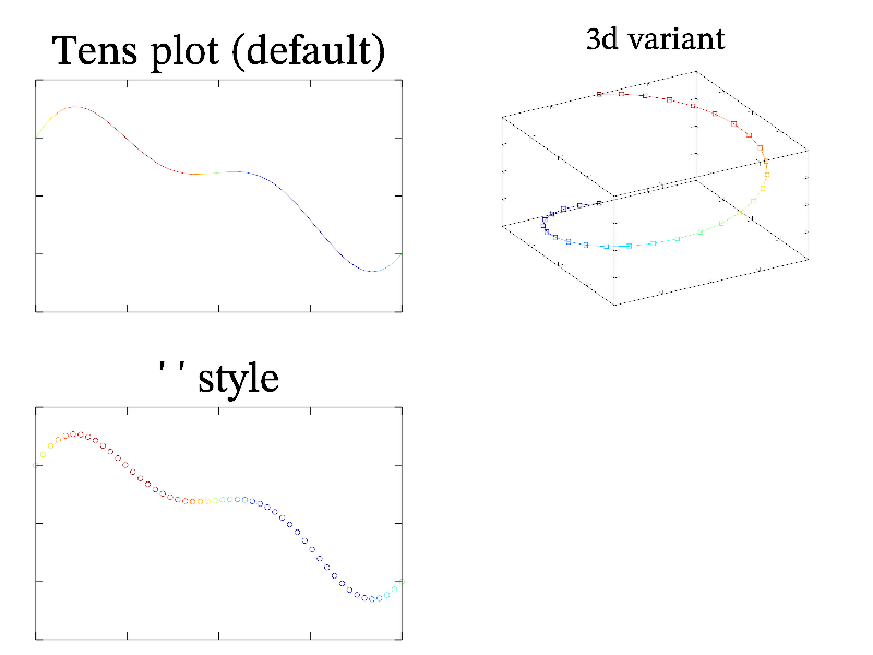
Next: text sample, Previous: tens sample, Up: All samples [Contents][Index]
Example of ternary coordinates.
MGL code:
ranges 0 1 0 1 0 1 new x 50 '0.25*(1+cos(2*pi*x))' new y 50 '0.25*(1+sin(2*pi*x))' new z 50 'x' new a 20 30 '30*x*y*(1-x-y)^2*(x+y<1)' new rx 10 'rnd':new ry 10:fill ry '(1-v)*rnd' rx light on subplot 2 2 0:title 'Ordinary axis 3D':rotate 50 60 box:axis:grid plot x y z 'r2':surf a '#' xlabel 'B':ylabel 'C':zlabel 'Z' subplot 2 2 1:title 'Ternary axis (x+y+t=1)':ternary 1 box:axis:grid 'xyz' 'B;' plot x y 'r2':plot rx ry 'q^ ':cont a:line 0.5 0 0 0.75 'g2' xlabel 'B':ylabel 'C':tlabel 'A' subplot 2 2 2:title 'Quaternary axis 3D':rotate 50 60:ternary 2 box:axis:grid 'xyz' 'B;' plot x y z 'r2':surf a '#' xlabel 'B':ylabel 'C':tlabel 'A':zlabel 'D' subplot 2 2 3:title 'Ternary axis 3D':rotate 50 60:ternary 1 box:axis:grid 'xyz' 'B;' plot x y z 'r2':surf a '#' xlabel 'B':ylabel 'C':tlabel 'A':zlabel 'Z'
C++ code:
void smgl_ternary(mglGraph *gr) // flag #
{
gr->SetRanges(0,1,0,1,0,1);
mglData x(50),y(50),z(50),rx(10),ry(10), a(20,30);
a.Modify("30*x*y*(1-x-y)^2*(x+y<1)");
x.Modify("0.25*(1+cos(2*pi*x))");
y.Modify("0.25*(1+sin(2*pi*x))");
rx.Modify("rnd"); ry.Modify("(1-v)*rnd",rx);
z.Modify("x");
gr->SubPlot(2,2,0); gr->Title("Ordinary axis 3D");
gr->Rotate(50,60); gr->Light(true);
gr->Plot(x,y,z,"r2"); gr->Surf(a,"BbcyrR#");
gr->Axis(); gr->Grid(); gr->Box();
gr->Label('x',"B",1); gr->Label('y',"C",1); gr->Label('z',"Z",1);
gr->SubPlot(2,2,1); gr->Title("Ternary axis (x+y+t=1)");
gr->Ternary(1);
gr->Plot(x,y,"r2"); gr->Plot(rx,ry,"q^ "); gr->Cont(a);
gr->Line(mglPoint(0.5,0), mglPoint(0,0.75), "g2");
gr->Axis(); gr->Grid("xyz","B;");
gr->Label('x',"B"); gr->Label('y',"C"); gr->Label('t',"A");
gr->SubPlot(2,2,2); gr->Title("Quaternary axis 3D");
gr->Rotate(50,60); gr->Light(true);
gr->Ternary(2);
gr->Plot(x,y,z,"r2"); gr->Surf(a,"BbcyrR#");
gr->Axis(); gr->Grid(); gr->Box();
gr->Label('t',"A",1); gr->Label('x',"B",1);
gr->Label('y',"C",1); gr->Label('z',"D",1);
gr->SubPlot(2,2,3); gr->Title("Ternary axis 3D");
gr->Rotate(50,60); gr->Light(true);
gr->Ternary(1);
gr->Plot(x,y,z,"r2"); gr->Surf(a,"BbcyrR#");
gr->Axis(); gr->Grid(); gr->Box();
gr->Label('t',"A",1); gr->Label('x',"B",1);
gr->Label('y',"C",1); gr->Label('z',"Z",1);
}
Next: text2 sample, Previous: ternary sample, Up: All samples [Contents][Index]
Example of text possibilities.
MGL code:
call 'prepare1d'
subplot 2 2 0 ''
text 0 1 'Text can be in ASCII and in Unicode'
text 0 0.6 'It can be \wire{wire}, \big{big} or #r{colored}'
text 0 0.2 'One can change style in string: \b{bold}, \i{italic, \b{both}}'
text 0 -0.2 'Easy to \a{overline} or \u{underline}'
text 0 -0.6 'Easy to change indexes ^{up} _{down} @{center}'
text 0 -1 'It parse TeX: \int \alpha \cdot \
\sqrt3{sin(\pi x)^2 + \gamma_{i_k}} dx'
subplot 2 2 1 ''
text 0 0.5 '\sqrt{\frac{\alpha^{\gamma^2}+\overset 1{\big\infty}}{\sqrt3{2+b}}}' '@' -2
text 0 -0.1 'More text position: \frac{a}{b}, \dfrac{a}{b}, [\stack{a}{bbb}], [\stackl{a}{bbb}], [\stackr{a}{bbb}], \sup{a}{sup}, \sub{a}{sub}'text 0 -0.5 'Text can be printed\n{}on several lines'
text 0 -0.9 'or with color gradient' 'BbcyrR'
subplot 2 2 2 '':box:plot y(:,0)
text y 'This is very very long string drawn along a curve' 'k'
text y 'Another string drawn above a curve' 'Tr'
subplot 2 2 3 '':line -1 -1 1 -1 'rA':text 0 -1 1 -1 'Horizontal'
line -1 -1 1 1 'rA':text 0 0 1 1 'At angle' '@'
line -1 -1 -1 1 'rA':text -1 0 -1 1 'Vertical'
C++ code:
void smgl_text(mglGraph *gr) // text drawing
{
if(big!=3) gr->SubPlot(2,2,0,"");
gr->Putsw(mglPoint(0,1),L"Text can be in ASCII and in Unicode");
gr->Puts(mglPoint(0,0.6),"It can be \\wire{wire}, \\big{big} or #r{colored}");
gr->Puts(mglPoint(0,0.2),"One can change style in string: "
"\\b{bold}, \\i{italic, \\b{both}}");
gr->Puts(mglPoint(0,-0.2),"Easy to \\a{overline} or "
"\\u{underline}");
gr->Puts(mglPoint(0,-0.6),"Easy to change indexes ^{up} _{down} @{center}");
gr->Puts(mglPoint(0,-1),"It parse TeX: \\int \\alpha \\cdot "
"\\sqrt3{sin(\\pi x)^2 + \\gamma_{i_k}} dx");
if(big==3) return;
gr->SubPlot(2,2,1,"");
gr->Puts(mglPoint(0,0.5), "\\sqrt{\\frac{\\alpha^{\\gamma^2}+\\overset 1{\\big\\infty}}{\\sqrt3{2+b}}}", "@", -2);
gr->Puts(mglPoint(0,-0.1),"More text position: \\frac{a}{b}, \\dfrac{a}{b}, [\\stack{a}{bbb}], [\\stackl{a}{bbb}], [\\stackr{a}{bbb}], \\sup{a}{sup}, \\sub{a}{sub}");
gr->Puts(mglPoint(0,-0.5),"Text can be printed\non several lines");
gr->Puts(mglPoint(0,-0.9),"or with col\bor gradient","BbcyrR");
gr->SubPlot(2,2,2,"");
mglData y; mgls_prepare1d(&y);
gr->Box(); gr->Plot(y.SubData(-1,0));
gr->Text(y,"This is very very long string drawn along a curve","k");
gr->Text(y,"Another string drawn under a curve","Tr");
gr->SubPlot(2,2,3,"");
gr->Line(mglPoint(-1,-1),mglPoint(1,-1),"rA"); gr->Puts(mglPoint(0,-1),mglPoint(1,-1),"Horizontal");
gr->Line(mglPoint(-1,-1),mglPoint(1,1),"rA"); gr->Puts(mglPoint(0,0),mglPoint(1,1),"At angle","@");
gr->Line(mglPoint(-1,-1),mglPoint(-1,1),"rA"); gr->Puts(mglPoint(-1,0),mglPoint(-1,1),"Vertical");
}
Next: textmark sample, Previous: text sample, Up: All samples [Contents][Index]
Example of text along curve.
MGL code:
call 'prepare1d' subplot 1 3 0 '':box:plot y(:,0) text y 'This is very very long string drawn along a curve' 'k' text y 'Another string drawn under a curve' 'Tr' subplot 1 3 1 '':box:plot y(:,0) text y 'This is very very long string drawn along a curve' 'k:C' text y 'Another string drawn under a curve' 'Tr:C' subplot 1 3 2 '':box:plot y(:,0) text y 'This is very very long string drawn along a curve' 'k:R' text y 'Another string drawn under a curve' 'Tr:R'
C++ code:
void smgl_text2(mglGraph *gr) // text drawing
{
mglData y; mgls_prepare1d(&y);
if(big!=3) gr->SubPlot(1,3,0,"");
gr->Box(); gr->Plot(y.SubData(-1,0));
gr->Text(y,"This is very very long string drawn along a curve","k");
gr->Text(y,"Another string drawn under a curve","Tr");
if(big==3) return;
gr->SubPlot(1,3,1,"");
gr->Box(); gr->Plot(y.SubData(-1,0));
gr->Text(y,"This is very very long string drawn along a curve","k:C");
gr->Text(y,"Another string drawn under a curve","Tr:C");
gr->SubPlot(1,3,2,"");
gr->Box(); gr->Plot(y.SubData(-1,0));
gr->Text(y,"This is very very long string drawn along a curve","k:R");
gr->Text(y,"Another string drawn under a curve","Tr:R");
}
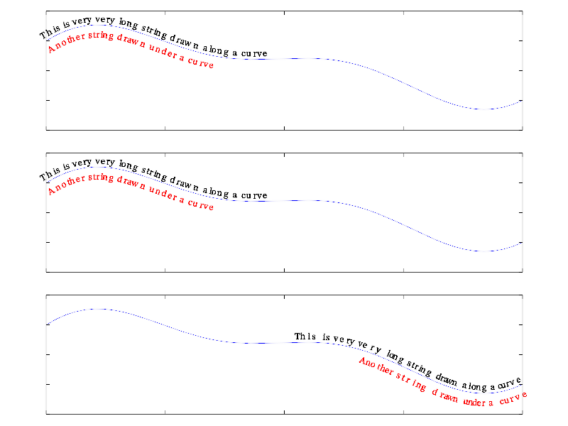
Next: ticks sample, Previous: text2 sample, Up: All samples [Contents][Index]
Function textmark is similar to mark but draw text instead of markers.
MGL code:
call 'prepare1d' subplot 1 1 0 '':title 'TextMark plot (default)':box:textmark y y1 '\gamma' 'r'
C++ code:
void smgl_textmark(mglGraph *gr)
{
mglData y,y1; mgls_prepare1d(&y,&y1);
if(big!=3) { gr->SubPlot(1,1,0,""); gr->Title("TextMark plot (default)"); }
gr->Box(); gr->TextMark(y,y1,"\\gamma","r");
}
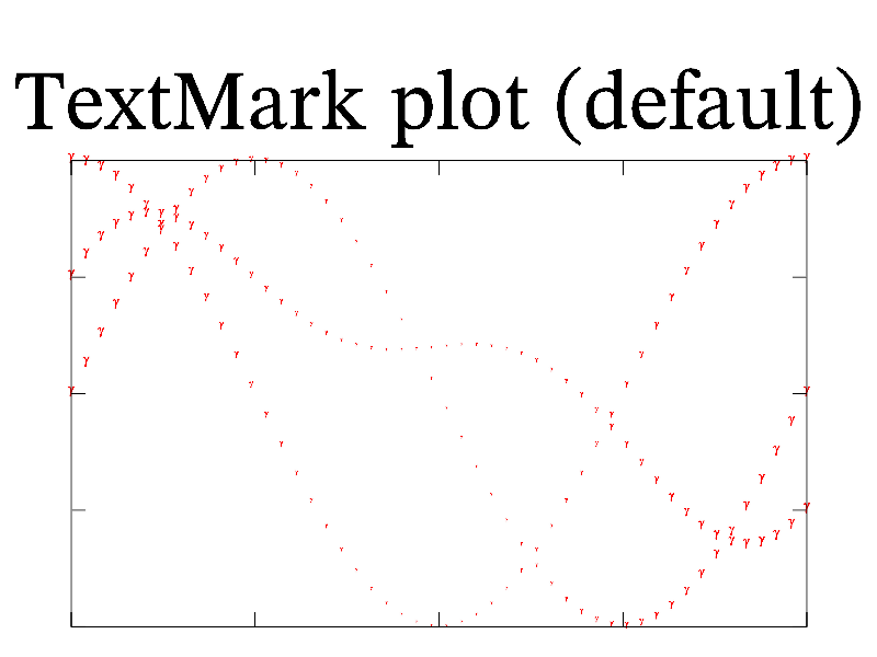
Next: tile sample, Previous: textmark sample, Up: All samples [Contents][Index]
Example of axis ticks.
MGL code:
subplot 3 3 0:title 'Usual axis with ":" style' axis ':' subplot 3 3 1:title 'Too big/small range' ranges -1000 1000 0 0.001:axis subplot 3 3 2:title 'LaTeX-like labels' axis 'F!' subplot 3 3 3:title 'Too narrow range' ranges 100 100.1 10 10.01:axis subplot 3 3 4:title 'No tuning, manual "+"' axis '+!' # for version <2.3 you can use #tuneticks off:axis subplot 3 3 5:title 'Template for ticks' xtick 'xxx:%g':ytick 'y:%g' axis xtick '':ytick '' # switch it off for other plots subplot 3 3 6:title 'No tuning, higher precision' axis '!4' subplot 3 3 7:title 'Manual ticks' ranges -pi pi 0 2 xtick pi 3 '\pi' xtick 0.886 'x^*' on # note this will disable subticks drawing # or you can use #xtick -pi '\pi' -pi/2 '-\pi/2' 0 '0' 0.886 'x^*' pi/2 '\pi/2' pi 'pi' list v 0 0.5 1 2:ytick v '0 0.5 1 2' axis:grid:fplot '2*cos(x^2)^2' 'r2' subplot 3 3 8:title 'Time ticks' xrange 0 3e5:ticktime 'x':axis
C++ code:
void smgl_ticks(mglGraph *gr)
{
gr->SubPlot(3,3,0); gr->Title("Usual axis with ':' style"); gr->Axis(":");
gr->SubPlot(3,3,1); gr->Title("Too big/small range");
gr->SetRanges(-1000,1000,0,0.001); gr->Axis();
gr->SubPlot(3,3,2); gr->Title("LaTeX-like labels");
gr->Axis("F!");
gr->SubPlot(3,3,3); gr->Title("Too narrow range");
gr->SetRanges(100,100.1,10,10.01); gr->Axis();
gr->SubPlot(3,3,4); gr->Title("No tuning, manual '+'");
// for version<2.3 you need first call gr->SetTuneTicks(0);
gr->Axis("+!");
gr->SubPlot(3,3,5); gr->Title("Template for ticks");
gr->SetTickTempl('x',"xxx:%g"); gr->SetTickTempl('y',"y:%g");
gr->Axis();
// now switch it off for other plots
gr->SetTickTempl('x',""); gr->SetTickTempl('y',"");
gr->SubPlot(3,3,6); gr->Title("No tuning, higher precision");
gr->Axis("!4");
gr->SubPlot(3,3,7); gr->Title("Manual ticks"); gr->SetRanges(-M_PI,M_PI, 0, 2);
gr->SetTicks('x',M_PI,0,0,"\\pi"); gr->AddTick('x',0.886,"x^*");
// alternatively you can use following lines
double val[]={0, 0.5, 1, 2};
gr->SetTicksVal('y', mglData(4,val), "0\n0.5\n1\n2");
gr->Axis(); gr->Grid(); gr->FPlot("2*cos(x^2)^2", "r2");
gr->SubPlot(3,3,8); gr->Title("Time ticks"); gr->SetRange('x',0,3e5);
gr->SetTicksTime('x',0); gr->Axis();
}
Next: tiles sample, Previous: ticks sample, Up: All samples [Contents][Index]
Function tile draw surface by tiles.
MGL code:
call 'prepare2d' title 'Tile plot':rotate 50 60:box:tile a
C++ code:
void smgl_tile(mglGraph *gr)
{
mglData a; mgls_prepare2d(&a);
if(big!=3) gr->Title("Tile plot");
gr->Rotate(40,60); gr->Box(); gr->Tile(a);
}
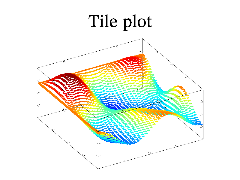
Next: torus sample, Previous: tile sample, Up: All samples [Contents][Index]
Function tiles is similar to tile but tile sizes is determined by another data. This allows one to simulate transparency of the plot.
MGL code:
call 'prepare2d' subplot 1 1 0 '':title 'Tiles plot':box:tiles a b
C++ code:
void smgl_tiles(mglGraph *gr)
{
mglData a,b; mgls_prepare2d(&a,&b);
if(big!=3) {gr->SubPlot(1,1,0,""); gr->Title("TileS plot");}
gr->Box(); gr->TileS(a,b);
}
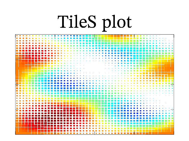
Next: traj sample, Previous: tiles sample, Up: All samples [Contents][Index]
Function torus draw surface of the curve rotation.
MGL code:
call 'prepare1d' subplot 2 2 0:title 'Torus plot (default)':light on:rotate 50 60:box:torus y1 y2 subplot 2 2 1:title '"x" style':light on:rotate 50 60:box:torus y1 y2 'x' subplot 2 2 2:title '"z" style':light on:rotate 50 60:box:torus y1 y2 'z' subplot 2 2 3:title '"\#" style':light on:rotate 50 60:box:torus y1 y2 '#'
C++ code:
void smgl_torus(mglGraph *gr)
{
mglData y1,y2; mgls_prepare1d(0,&y1,&y2);
if(big!=3) { gr->SubPlot(2,2,0); gr->Title("Torus plot (default)"); }
gr->Light(true); gr->Rotate(50,60); gr->Box(); gr->Torus(y1,y2);
if(big==3) return;
gr->SubPlot(2,2,1); gr->Title("'x' style"); gr->Rotate(50,60); gr->Box(); gr->Torus(y1,y2,"x");
gr->SubPlot(2,2,2); gr->Title("'z' style"); gr->Rotate(50,60); gr->Box(); gr->Torus(y1,y2,"z");
gr->SubPlot(2,2,3); gr->Title("'\\#' style"); gr->Rotate(50,60); gr->Box(); gr->Torus(y1,y2,"#");
}
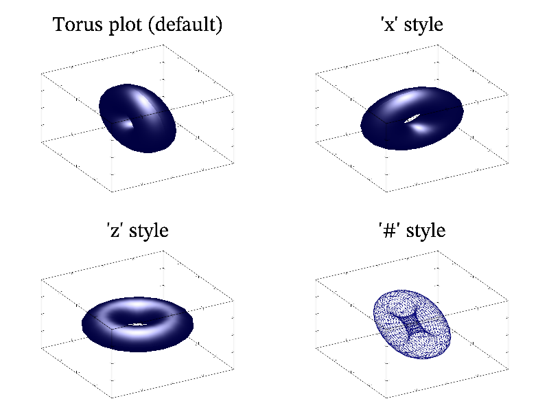
Next: triangulation sample, Previous: torus sample, Up: All samples [Contents][Index]
Function traj is 1D analogue of vect. It draw vectors from specified points.
MGL code:
call 'prepare1d' subplot 1 1 0 '':title 'Traj plot':box:plot x1 y:traj x1 y y1 y2
C++ code:
void smgl_traj(mglGraph *gr)
{
mglData x,y,y1,y2; mgls_prepare1d(&y,&y1,&y2,&x);
if(big!=3) {gr->SubPlot(1,1,0,""); gr->Title("Traj plot");}
gr->Box(); gr->Plot(x,y); gr->Traj(x,y,y1,y2);
}

Next: triplot sample, Previous: traj sample, Up: All samples [Contents][Index]
Example of use triangulate for arbitrary placed points.
MGL code:
new x 100 '2*rnd-1':new y 100 '2*rnd-1':copy z x^2-y^2 new g 30 30:triangulate d x y title 'Triangulation' rotate 50 60:box:light on triplot d x y z:triplot d x y z '#k' datagrid g x y z:mesh g 'm'
C++ code:
void smgl_triangulation(mglGraph *gr) // surface triangulation
{
mglData x(100), y(100), z(100);
gr->Fill(x,"2*rnd-1"); gr->Fill(y,"2*rnd-1"); gr->Fill(z,"v^2-w^2",x,y);
mglData d = mglTriangulation(x,y), g(30,30);
if(big!=3) gr->Title("Triangulation");
gr->Rotate(40,60); gr->Box(); gr->Light(true);
gr->TriPlot(d,x,y,z); gr->TriPlot(d,x,y,z,"#k");
gr->DataGrid(g,x,y,z); gr->Mesh(g,"m");
}
Next: tube sample, Previous: triangulation sample, Up: All samples [Contents][Index]
Functions triplot and quadplot draw set of triangles (or quadrangles, correspondingly) for irregular data arrays. Note, that you have to provide not only vertexes, but also the indexes of triangles or quadrangles. I.e. perform triangulation by some other library. See also triangulate.
MGL code:
list q 0 1 2 3 | 4 5 6 7 | 0 2 4 6 | 1 3 5 7 | 0 4 1 5 | 2 6 3 7 list xq -1 1 -1 1 -1 1 -1 1 list yq -1 -1 1 1 -1 -1 1 1 list zq -1 -1 -1 -1 1 1 1 1 light on subplot 2 2 0:title 'QuadPlot sample':rotate 50 60 quadplot q xq yq zq 'yr' quadplot q xq yq zq '#k' subplot 2 2 2:title 'QuadPlot coloring':rotate 50 60 quadplot q xq yq zq yq 'yr' quadplot q xq yq zq '#k' list t 0 1 2 | 0 1 3 | 0 2 3 | 1 2 3 list xt -1 1 0 0 list yt -1 -1 1 0 list zt -1 -1 -1 1 subplot 2 2 1:title 'TriPlot sample':rotate 50 60 triplot t xt yt zt 'b' triplot t xt yt zt '#k' subplot 2 2 3:title 'TriPlot coloring':rotate 50 60 triplot t xt yt zt yt 'cb' triplot t xt yt zt '#k' tricont t xt yt zt 'B'
C++ code:
void smgl_triplot(mglGraph *gr)
{
double q[] = {0,1,2,3, 4,5,6,7, 0,2,4,6, 1,3,5,7, 0,4,1,5, 2,6,3,7};
double xc[] = {-1,1,-1,1,-1,1,-1,1}, yc[] = {-1,-1,1,1,-1,-1,1,1}, zc[] = {-1,-1,-1,-1,1,1,1,1};
mglData qq(6,4,q), xx(8,xc), yy(8,yc), zz(8,zc);
gr->Light(true); //gr->Alpha(true);
gr->SubPlot(2,2,0); gr->Title("QuadPlot sample"); gr->Rotate(50,60);
gr->QuadPlot(qq,xx,yy,zz,"yr");
gr->QuadPlot(qq,xx,yy,zz,"k#");
gr->SubPlot(2,2,2); gr->Title("QuadPlot coloring"); gr->Rotate(50,60);
gr->QuadPlot(qq,xx,yy,zz,yy,"yr");
gr->QuadPlot(qq,xx,yy,zz,"k#");
double t[] = {0,1,2, 0,1,3, 0,2,3, 1,2,3};
double xt[] = {-1,1,0,0}, yt[] = {-1,-1,1,0}, zt[] = {-1,-1,-1,1};
mglData tt(4,3,t), uu(4,xt), vv(4,yt), ww(4,zt);
gr->SubPlot(2,2,1); gr->Title("TriPlot sample"); gr->Rotate(50,60);
gr->TriPlot(tt,uu,vv,ww,"b");
gr->TriPlot(tt,uu,vv,ww,"k#");
gr->SubPlot(2,2,3); gr->Title("TriPlot coloring"); gr->Rotate(50,60);
gr->TriPlot(tt,uu,vv,ww,vv,"cb");
gr->TriPlot(tt,uu,vv,ww,"k#");
gr->TriCont(tt,uu,vv,ww,"B");
}
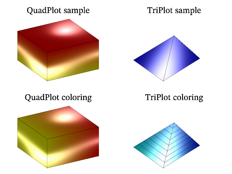
Next: type0 sample, Previous: triplot sample, Up: All samples [Contents][Index]
Function tube draw tube with variable radius.
MGL code:
call 'prepare1d' light on new yc 50 'sin(pi*x)':new xc 50 'cos(pi*x)':new z 50 'x':divto y1 20 subplot 2 2 0 '':title 'Tube plot (default)':box:tube y 0.05 subplot 2 2 1 '':title 'variable radius':box:tube y y1 subplot 2 2 2 '':title '"\#" style':box:tube y 0.05 '#' subplot 2 2 3:title '3d variant':rotate 50 60:box:tube xc yc z y2 'r'
C++ code:
void smgl_tube(mglGraph *gr)
{
mglData y,y1,y2; mgls_prepare1d(&y,&y1,&y2); y1/=20;
if(big!=3) { gr->SubPlot(2,2,0,""); gr->Title("Tube plot (default)"); }
gr->Light(true); gr->Box(); gr->Tube(y,0.05);
if(big==3) return;
gr->SubPlot(2,2,1,""); gr->Title("variable radius"); gr->Box(); gr->Tube(y,y1);
gr->SubPlot(2,2,2,""); gr->Title("'\\#' style"); gr->Box(); gr->Tube(y,0.05,"#");
mglData yc(50), xc(50), z(50); z.Modify("2*x-1");
yc.Modify("sin(pi*(2*x-1))"); xc.Modify("cos(pi*2*x-pi)");
gr->SubPlot(2,2,3); gr->Title("3d variant"); gr->Rotate(50,60); gr->Box(); gr->Tube(xc,yc,z,y2,"r");
}
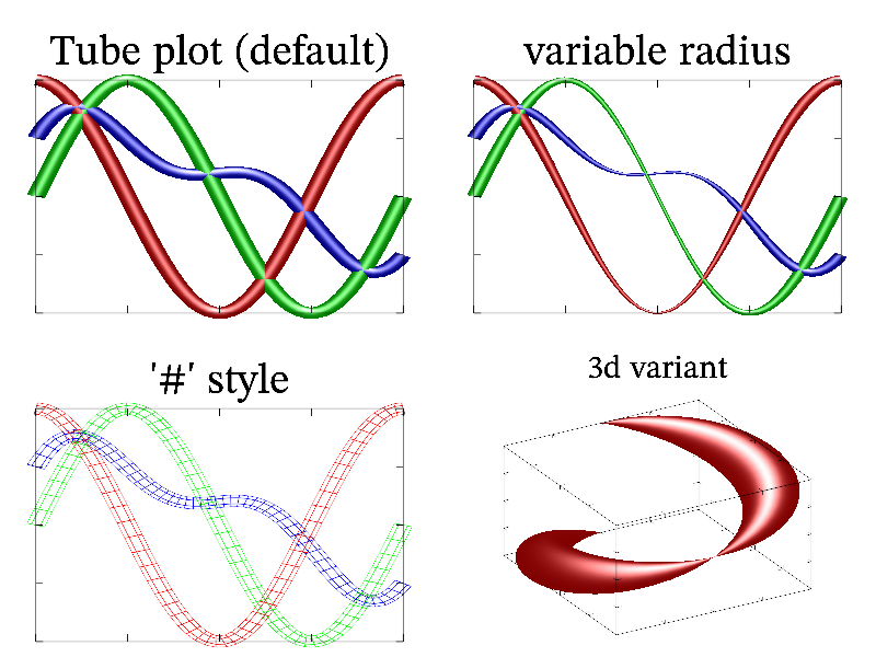
Next: type1 sample, Previous: tube sample, Up: All samples [Contents][Index]
Example of ordinary transparency (transptype=0).
MGL code:
call 'prepare2d' alpha on:light on:transptype 0:clf subplot 2 2 0:rotate 50 60:surf a:box subplot 2 2 1:rotate 50 60:dens a:box subplot 2 2 2:rotate 50 60:cont a:box subplot 2 2 3:rotate 50 60:axial a:box
C++ code:
void smgl_type0(mglGraph *gr) // TranspType = 0
{
gr->Alpha(true); gr->Light(true);
mglData a; mgls_prepare2d(&a);
gr->SetTranspType(0); gr->Clf();
gr->SubPlot(2,2,0); gr->Rotate(50,60); gr->Surf(a); gr->Box();
gr->SubPlot(2,2,1); gr->Rotate(50,60); gr->Dens(a); gr->Box();
gr->SubPlot(2,2,2); gr->Rotate(50,60); gr->Cont(a); gr->Box();
gr->SubPlot(2,2,3); gr->Rotate(50,60); gr->Axial(a); gr->Box();
}
Next: type2 sample, Previous: type0 sample, Up: All samples [Contents][Index]
Example of glass-like transparency (transptype=1).
MGL code:
call 'prepare2d' alpha on:light on:transptype 1:clf subplot 2 2 0:rotate 50 60:surf a:box subplot 2 2 1:rotate 50 60:dens a:box subplot 2 2 2:rotate 50 60:cont a:box subplot 2 2 3:rotate 50 60:axial a:box
C++ code:
void smgl_type1(mglGraph *gr) // TranspType = 1
{
gr->Alpha(true); gr->Light(true);
mglData a; mgls_prepare2d(&a);
gr->SetTranspType(1); gr->Clf();
gr->SubPlot(2,2,0); gr->Rotate(50,60); gr->Surf(a); gr->Box();
gr->SubPlot(2,2,1); gr->Rotate(50,60); gr->Dens(a); gr->Box();
gr->SubPlot(2,2,2); gr->Rotate(50,60); gr->Cont(a); gr->Box();
gr->SubPlot(2,2,3); gr->Rotate(50,60); gr->Axial(a); gr->Box();
}
Next: vect sample, Previous: type1 sample, Up: All samples [Contents][Index]
Example of lamp-like transparency (transptype=2).
MGL code:
call 'prepare2d' alpha on:light on:transptype 2:clf subplot 2 2 0:rotate 50 60:surf a:box subplot 2 2 1:rotate 50 60:dens a:box subplot 2 2 2:rotate 50 60:cont a:box subplot 2 2 3:rotate 50 60:axial a:box
C++ code:
void smgl_type2(mglGraph *gr) // TranspType = 2
{
gr->Alpha(true); gr->Light(true);
mglData a; mgls_prepare2d(&a);
gr->SetTranspType(2); gr->Clf();
gr->SubPlot(2,2,0); gr->Rotate(50,60); gr->Surf(a); gr->Box();
gr->SubPlot(2,2,1); gr->Rotate(50,60); gr->Dens(a); gr->Box();
gr->SubPlot(2,2,2); gr->Rotate(50,60); gr->Cont(a); gr->Box();
gr->SubPlot(2,2,3); gr->Rotate(50,60); gr->Axial(a); gr->Box();
}
Next: vect3 sample, Previous: type2 sample, Up: All samples [Contents][Index]
Function vect is most standard way to visualize vector fields – it draw a lot of arrows or hachures for each data cell. It have a lot of options which can be seen on the figure (and in the sample code), and use color scheme for coloring (see Color scheme).
MGL code:
call 'prepare2v' call 'prepare3v' subplot 3 2 0 '':title 'Vect plot (default)':box:vect a b subplot 3 2 1 '':title '"." style; "=" style':box:vect a b '.=' subplot 3 2 2 '':title '"f" style':box:vect a b 'f' subplot 3 2 3 '':title '">" style':box:vect a b '>' subplot 3 2 4 '':title '"<" style':box:vect a b '<' subplot 3 2 5:title '3d variant':rotate 50 60:box:vect ex ey ez
C++ code:
void smgl_vect3(mglGraph *gr)
{
mglData ex,ey,ez; mgls_prepare3v(&ex,&ey,&ez);
if(big!=3) { gr->SubPlot(2,1,0); gr->Title("Vect3 sample"); }
gr->Rotate(50,60); gr->SetOrigin(0,0,0); gr->Axis("_xyz"); gr->Box();
gr->Vect3(ex,ey,ez,"x"); gr->Vect3(ex,ey,ez); gr->Vect3(ex,ey,ez,"z");
if(big==3) return;
gr->SubPlot(2,1,1); gr->Title("'f' style");
gr->Rotate(50,60); gr->SetOrigin(0,0,0); gr->Axis("_xyz"); gr->Box();
gr->Vect3(ex,ey,ez,"fx"); gr->Vect3(ex,ey,ez,"f"); gr->Vect3(ex,ey,ez,"fz");
gr->Grid3(ex,"Wx"); gr->Grid3(ex,"W"); gr->Grid3(ex,"Wz");
}
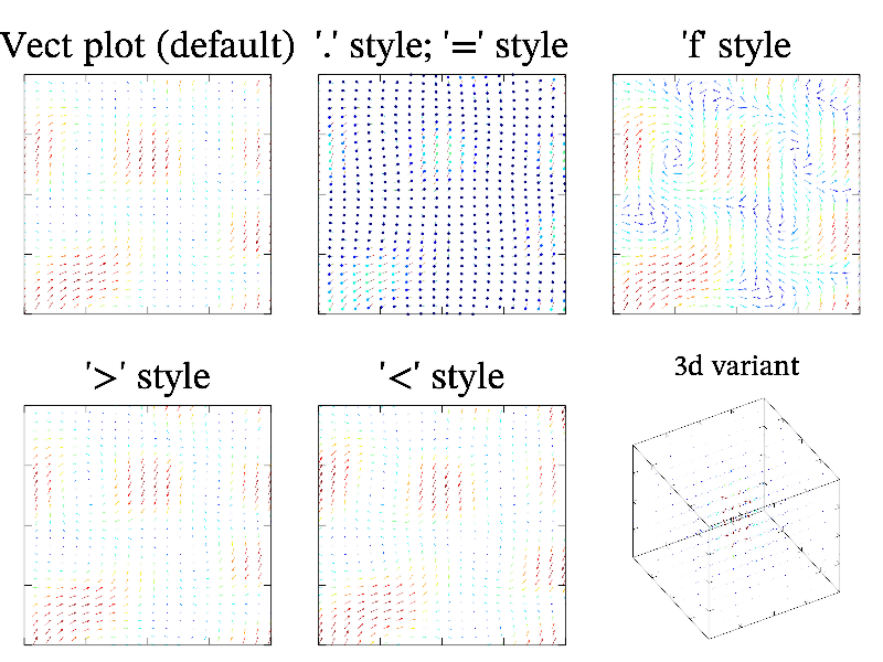
Next: venn sample, Previous: vect sample, Up: All samples [Contents][Index]
Function vect3 draw ordinary vector field plot but at slices of 3D data.
MGL code:
call 'prepare3v' subplot 2 1 0:title 'Vect3 sample':rotate 50 60 origin 0 0 0:box:axis '_xyz' vect3 ex ey ez 'x':vect3 ex ey ez:vect3 ex ey ez 'z' subplot 2 1 1:title '"f" style':rotate 50 60 origin 0 0 0:box:axis '_xyz' vect3 ex ey ez 'fx':vect3 ex ey ez 'f':vect3 ex ey ez 'fz' grid3 ex 'Wx':grid3 ex 'W':grid3 ex 'Wz'
C++ code:
void smgl_vect3(mglGraph *gr)
{
mglData ex,ey,ez; mgls_prepare3v(&ex,&ey,&ez);
if(big!=3) { gr->SubPlot(2,1,0); gr->Title("Vect3 sample"); }
gr->Rotate(50,60); gr->SetOrigin(0,0,0); gr->Axis("_xyz"); gr->Box();
gr->Vect3(ex,ey,ez,"x"); gr->Vect3(ex,ey,ez); gr->Vect3(ex,ey,ez,"z");
if(big==3) return;
gr->SubPlot(2,1,1); gr->Title("'f' style");
gr->Rotate(50,60); gr->SetOrigin(0,0,0); gr->Axis("_xyz"); gr->Box();
gr->Vect3(ex,ey,ez,"fx"); gr->Vect3(ex,ey,ez,"f"); gr->Vect3(ex,ey,ez,"fz");
gr->Grid3(ex,"Wx"); gr->Grid3(ex,"W"); gr->Grid3(ex,"Wz");
}
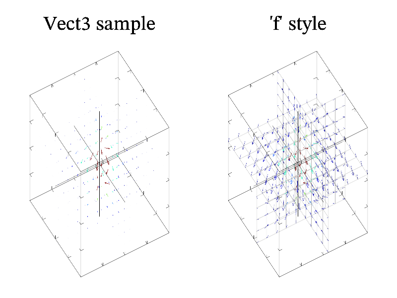
Previous: vect3 sample, Up: All samples [Contents][Index]
Example of venn-like diagram.
MGL code:
list x -0.3 0 0.3:list y 0.3 -0.3 0.3:list e 0.7 0.7 0.7 subplot 1 1 0:title 'Venn-like diagram' transptype 1:alpha on:error x y e e '!rgb@#o';alpha 0.1
C++ code:
void smgl_venn(mglGraph *gr)
{
double xx[3]={-0.3,0,0.3}, yy[3]={0.3,-0.3,0.3}, ee[3]={0.7,0.7,0.7};
mglData x(3,xx), y(3,yy), e(3,ee);
gr->SubPlot(1,1,0); gr->Title("Venn-like diagram");
gr->SetTranspType(1); gr->Alpha(true); gr->Error(x,y,e,e,"!rgb@#o","alpha 0.1");
}
Next: File formats, Previous: All samples, Up: Top [Contents][Index]
This appendix contain the full list of symbols (characters) used by MathGL for setting up plot. Also it contain sections for full list of hot-keys supported by mglview tool and by UDAV program.
| • Symbols for styles | ||
| • Hot-keys for mglview | ||
| • Hot-keys for UDAV |
Next: Hot-keys for mglview, Up: Symbols and hot-keys [Contents][Index]
Below is full list of all characters (symbols) which MathGL use for setting up the plot.
empty line style (see Line styles);
empty color in chart.
set to use new color from palette for each point (not for each curve, as default) in 1D plotting;
set to disable ticks tuning in axis and colorbar;
set to draw grid lines at subticks coordinates too;
define complex variable/expression in MGL script if placed at beginning.
set to use solid marks (see Line styles) or solid error boxes;
set to draw wired plot for axial, surf3, surf3a, surf3c, triplot, quadplot, area, region, bars, barh, tube, tape, cone, boxs and draw boundary only for circle, ellipse, rhomb;
set to draw also mesh lines for surf, surfc, surfa, dens, densx, densy, densz, dens3, or boundary for chart, facex, facey, facez, rect;
set to draw boundary and box for legend, title, or grid lines for table;
set to draw grid for radar;
set to start flow threads and pipes from edges only for flow, pipe;
set to use whole are for axis range in subplot, inplot;
change text color inside a string (see Font styles);
start comment in MGL scripts or in Command options.
denote parameter of MGL scripts.
set color scheme along 2 coordinates Color scheme;
operation in Textual formulas.
set to pass long integer number in tick template xtick, ytick, ztick, ctick;
specifier of drawing user-defined symbols as mark (see Line styles);
operation in Textual formulas.
denote string in MGL scripts or in Command options.
one of marks (see Line styles);
one of mask for face filling (see Color scheme);
set to start flow threads from 2d array inside data (see flow);
operation in Textual formulas.
one of marks (see Line styles) or kind of error boxes;
one of mask for face filling (see Color scheme);
set to print ‘+’ for positive numbers in axis, label, table;
operation of increasing last character value in MGL strings;
operation in Textual formulas.
separator for color positions (see Color styles) or items in a list
concatenation of MGL string with another string or numerical value.
solid line style (see Line styles);
one of mask for face filling (see Color scheme);
place entries horizontally in legend;
set to use usual ‘-’ for negative numbers in axis, label, table;
operation in Textual formulas.
one of marks (see Line styles) or kind of error boxes;
set to draw hachures instead of arrows for vect, vect3;
set to use dots instead of faces for cloud, torus, axial, surf3, surf3a, surf3c, surf, surfa, surfc, dens, map;
delimiter of fractional parts for numbers.
operation in Textual formulas.
line dashing style (see Line styles);
stop color scheme parsing (see Color scheme);
range operation in MGL scripts;
style for axis;
separator of commands in MGL scripts.
line dashing style (see Line styles);
one of mask for face filling (see Color scheme);
start of an option in MGL scripts or in Command options;
separator of equations in ode;
separator of labels in iris.
one of marks (see Line styles);
one of mask for face filling (see Color scheme);
set position of colorbar;
align left in bars, barh, boxplot, cones, candle, ohlc;
operation in Textual formulas.
one of marks (see Line styles);
one of mask for face filling (see Color scheme);
set position of colorbar;
align right in bars, barh, boxplot, cones, candle, ohlc;
operation in Textual formulas.
line dashing style (see Line styles);
one of mask for face filling (see Color scheme);
set to use equidistant columns for table;
set to use color gradient for vect, vect3;
operation in Textual formulas.
set to draw box around text for text and similar functions;
set to draw boundary and fill it for circle, ellipse, rhomb;
set to fill faces for box;
set to draw large semitransparent mark instead of error box for error;
set to draw edges for cone;
set to draw filled boxes for boxs;
reduce text size inside a string (see Font styles);
operation in Textual formulas.
one of marks (see Line styles);
one of mask for face filling (see Color scheme);
set position of colorbar;
set outer position for legend;
inverse default position for axis;
switch to upper index inside a string (see Font styles);
align center in bars, barh, boxplot, cones, candle, ohlc;
operation in Textual formulas.
empty arrow style (see Line styles);
disable drawing of tick labels for axis;
set position of colorbar;
set to draw contours at bottom for cont, contf, contd, contv, tricont;
switch to lower index inside a string (see Font styles).
contain symbols excluded from color scheme parsing (see Color scheme);
operation of getting n-th character from MGL string.
contain extended specification of color (see Color styles), dashing (see Line styles) or mask (see Color scheme);
denote special operation in MGL scripts;
denote ’meta-symbol’ for LaTeX like string parsing (see Font styles).
line dashing style (see Line styles);
set to use sharp color scheme (see Color scheme);
set to limit width by subplot width for table;
delimiter in list command;
operation in Textual formulas.
string continuation symbol on next line for MGL scripts.
disable drawing of tick labels for axis and colorbar;
disable first segment in lamerey;
reduce number of segments in plot and tens;
one of mask for face filling (see Color scheme).
line width (see Line styles);
brightness of a color (see Color styles);
precision of numbers in axis, label, table;
kind of smoothing (for digits 1,3,5) in smooth;
digits for a value.
set to draw square, hex- or octo-pyramids instead of cones in cone, cones.
can be hex-digit for color specification if placed inside {} (see Color styles).
arrow style (see Line styles);
set to use absolute position in whole picture for text, colorbar, legend.
set to use absolute position in subplot for text;
style of plot, radar, tens, area, region to draw segments between points outside of axis range;
dark blue color (see Color styles).
blue color (see Color styles);
bold font face if placed after ‘:’ (see Font styles).
dark cyan color (see Color styles);
align text to center if placed after ‘:’ (see Font styles).
cyan color (see Color styles);
name of color axis;
cosine transform for transform.
arrow style (see Line styles);
one of mask for face filling (see Color scheme).
one of marks (see Line styles) or kind of error boxes;
one of mask for face filling (see Color scheme);
start hex-dash description if placed inside {} (see Line styles).
dark green-yellow color (see Color styles).
green-yellow color (see Color styles).
set fixed format for numbers in axis, label, table;
Fourier transform for transform.
dark green color (see Color styles).
green color (see Color styles).
dark gray color (see Color styles).
gray color (see Color styles);
Hankel transform for transform.
arrow style (see Line styles);
set colorbar position near boundary.
line dashing style (see Line styles);
italic font face if placed after ‘:’ (see Font styles).
set to use inverse values for cloud, pipe, dew;
set to fill only area with y1<y<y2 for region;
inverse Fourier transform for transform, transforma, fourier.
line dashing style (see Line styles);
one of mask for face filling (see Color scheme).
arrow style (see Line styles).
black color (see Color styles).
dark green-blue color (see Color styles);
align text to left if placed after ‘:’ (see Font styles).
green-blue color (see Color styles).
dark magenta color (see Color styles).
magenta color (see Color styles).
dark sky-blue color (see Color styles).
sky-blue color (see Color styles).
arrow style (see Line styles);
one of mask for face filling (see Color scheme).
one of marks (see Line styles) or kind of error boxes;
one of mask for face filling (see Color scheme);
over-line text if placed after ‘:’ (see Font styles).
dark purple color (see Color styles).
purple color (see Color styles).
dark orange or brown color (see Color styles).
orange color (see Color styles).
dark red color (see Color styles);
align text to right if placed after ‘:’ (see Font styles).
red color (see Color styles).
arrow style (see Line styles);
one of mask for face filling (see Color scheme).
one of marks (see Line styles) or kind of error boxes;
one of mask for face filling (see Color scheme);
start hex-mask description if placed inside {} (see Color scheme);
sine transform for transform.
arrow style (see Line styles);
set to draw text labels for cont, cont3;
name of t-axis (one of ternary axis);
variable in Textual formulas, which usually is varied in range [0,1].
dark blue-violet color (see Color styles);
disable rotation of tick labels for axis.
blue-violet color (see Color styles);
under-line text if placed after ‘:’ (see Font styles);
name of u-axis (one of ternary axis);
variable in Textual formulas, which usually denote array itself.
arrow style (see Line styles);
place text centering on vertical direction for text.
one of marks (see Line styles);
set to draw vectors on flow threads for flow and on segments for lamerey.
bright gray color (see Color styles).
white color (see Color styles);
wired text if placed after ‘:’ (see Font styles);
name of w-axis (one of ternary axis);
arrow style (see Line styles).
name of x-axis or x-direction or 1st dimension of a data array;
start hex-color description if placed inside {} (see Color styles);
one of marks (see Line styles) or kind of error boxes;
tiles orientation perpendicular to x-axis in tile, tiles;
style of tape.
dark yellow or gold color (see Color styles).
yellow color (see Color styles);
name of y-axis or y-direction or 2nd dimension of a data array;
name of z-axis or z-direction or 3d dimension of a data array;
style of tape.
Next: Hot-keys for UDAV, Previous: Symbols for styles, Up: Symbols and hot-keys [Contents][Index]
| Key | Description |
|---|---|
| Ctrl-P | Open printer dialog and print graphics. |
| Ctrl-W | Close window. |
| Ctrl-T | Switch on/off transparency for the graphics. |
| Ctrl-L | Switch on/off additional lightning for the graphics. |
| Ctrl-Space | Restore default graphics rotation, zoom and perspective. |
| F5 | Execute script and redraw graphics. |
| F6 | Change canvas size to fill whole region. |
| F7 | Stop drawing and script execution. |
| Ctrl-F5 | Run slideshow. If no parameter specified then the dialog with slideshow options will appear. |
| Ctrl-Comma, Ctrl-Period | Show next/previous slide. If no parameter specified then the dialog with slideshow options will appear. |
| Ctrl-Shift-G | Copy graphics to clipboard. |
| Alt-P | Export as semitransparent PNG. |
| Alt-F | Export as solid PNG. |
| Alt-J | Export as JPEG. |
| Alt-E | Export as vector EPS. |
| Alt-S | Export as vector SVG. |
| Alt-L | Export as LaTeX/Tikz image. |
| Alt-M | Export as MGLD. |
| Alt-D | Export as PRC/PDF. |
| Alt-O | Export as OBJ. |
Previous: Hot-keys for mglview, Up: Symbols and hot-keys [Contents][Index]
| Key | Description |
|---|---|
| Ctrl-N | Create new window with empty script. Note, all scripts share variables. So, second window can be used to see some additional information of existed variables. |
| Ctrl-O | Open and execute/show script or data from file. You may switch off automatic exection in UDAV properties |
| Ctrl-S | Save script to a file. |
| Ctrl-P | Open printer dialog and print graphics. |
| Ctrl-Z | Undo changes in script editor. |
| Ctrl-Shift-Z | Redo changes in script editor. |
| Ctrl-X | Cut selected text into clipboard. |
| Ctrl-C | Copy selected text into clipboard. |
| Ctrl-V | Paste selected text from clipboard. |
| Ctrl-A | Select all text in editor. |
| Ctrl-F | Show dialog for text finding. |
| F3 | Find next occurrence of the text. |
| Win-C or Meta-C | Show dialog for new command and put it into the script. |
| Win-F or Meta-F | Insert last fitted formula with found coefficients. |
| Win-S or Meta-S | Show dialog for styles and put it into the script. Styles define the plot view (color scheme, marks, dashing and so on). |
| Win-O or Meta-O | Show dialog for options and put it into the script. Options are used for additional setup the plot. |
| Win-N or Meta-N | Replace selected expression by its numerical value. |
| Win-P or Meta-P | Select file and insert its file name into the script. |
| Win-G or Meta-G | Show dialog for plot setup and put resulting code into the script. This dialog setup axis, labels, lighting and other general things. |
| Ctrl-Shift-O | Load data from file. Data will be deleted only at exit but UDAV will not ask to save it. |
| Ctrl-Shift-S | Save data to a file. |
| Ctrl-Shift-C | Copy range of numbers to clipboard. |
| Ctrl-Shift-V | Paste range of numbers from clipboard. |
| Ctrl-Shift-N | Recreate the data with new sizes and fill it by zeros. |
| Ctrl-Shift-R | Resize (interpolate) the data to specified sizes. |
| Ctrl-Shift-T | Transform data along dimension(s). |
| Ctrl-Shift-M | Make another data. |
| Ctrl-Shift-H | Find histogram of data. |
| Ctrl-T | Switch on/off transparency for the graphics. |
| Ctrl-L | Switch on/off additional lightning for the graphics. |
| Ctrl-G | Switch on/off grid of absolute coordinates. |
| Ctrl-Space | Restore default graphics rotation, zoom and perspective. |
| F5 | Execute script and redraw graphics. |
| F6 | Change canvas size to fill whole region. |
| F7 | Stop script execution and drawing. |
| F8 | Show/hide tool window with list of hidden plots. |
| F9 | Restore status for ’once’ command and reload data. |
| Ctrl-F5 | Run slideshow. If no parameter specified then the dialog with slideshow options will appear. |
| Ctrl-Comma, Ctrl-Period | Show next/previous slide. If no parameter specified then the dialog with slideshow options will appear. |
| Ctrl-W | Open dialog with slideshow options. |
| Ctrl-Shift-G | Copy graphics to clipboard. |
| F1 | Show help on MGL commands |
| F2 | Show/hide tool window with messages and information. |
| F4 | Show/hide calculator which evaluate and help to type textual formulas. Textual formulas may contain data variables too. |
| Meta-Shift-Up, Meta-Shift-Down | Change view angle \theta. |
| Meta-Shift-Left, Meta-Shift-Right | Change view angle \phi. |
| Alt-Minus, Alt-Equal | Zoom in/out whole image. |
| Alt-Up, Alt-Down, Alt-Right, Alt-Left | Shift whole image. |
| Alt-P | Export as semitransparent PNG. |
| Alt-F | Export as solid PNG. |
| Alt-J | Export as JPEG. |
| Alt-E | Export as vector EPS. |
| Alt-S | Export as vector SVG. |
| Alt-L | Export as LaTeX/Tikz image. |
| Alt-M | Export as MGLD. |
| Alt-D | Export as PRC/PDF. |
| Alt-O | Export as OBJ. |
Next: Plotting time, Previous: Symbols and hot-keys, Up: Top [Contents][Index]
This appendix contain description of file formats used by MathGL.
| • Font files | ||
| • MGLD format | ||
| • JSON format | ||
| • IFS format |
Next: MGLD format, Up: File formats [Contents][Index]
Starting from v.1.6 the MathGL library uses new font files. The font is defined in 4 files with suffixes ‘*.vfm’, ‘*_b.vfm’, ‘*_i.vfm’, ‘*_bi.vfm’. These files are text files containing the data for roman font, bold font, italic font and bold italic font. The files (or some symbols in the files) for bold, italic or bold italic fonts can be absent. In this case the roman glyph will be used for them. By analogy, if the bold italic font is absent but the bold font is present then bold glyph will be used for bold italic. You may create these font files by yourself from *.ttf, *.otf files with the help of program font_tools. This program can be found at MathGL home site.
The format of font files (*.vfm – vector font for MathGL) is the following.
Each font file can be compressed by gzip.
Note: the closing contour line is done automatically (so the last segment may be absent). For starting new contour use a point with coordinates {0x3fff, 0x3fff}.
Next: JSON format, Previous: Font files, Up: File formats [Contents][Index]
MGLD is textual file, which contain all required information for drawing 3D image, i.e. it contain vertexes with colors and normales, primitives with all properties, textures, and glyph descriptions. MGLD file can be imported or viewed separately, without parsing data files itself.
MGLD file start from string
MGLD npnts nprim ntxtr nglfs # optional description
which contain signature ‘MGLD’ and number of points npnts, number of primitives nprim, number of textures ntxtr, number of glyph descriptions nglfs, and optional description. Empty strings and string with ‘#’ are ignored.
Next, file contain npnts strings with points coordinates and colors. The format of each string is
x y z c t ta u v w r g b a
Here x, y, z are coordinates, c, t are color indexes in texture, ta is normalized t according to current alpha setting, u, v, w are coordinates of normal vector (can be NAN if disabled), r, g, b, a are RGBA color values.
Next, file contain nprim strings with properties of primitives. The format of each string is
type n1 n2 n3 n4 id s w p
Here type is kind of primitive (0 - mark, 1 - line, 2 - triangle, 3 - quadrangle, 4 - glyph), n1...n4 is index of point for vertexes, id is primitive identification number, s and w are size and width if applicable, p is scaling factor for glyphs.
Next, file contain ntxtr strings with descriptions of textures. The format of each string is
smooth alpha colors
Here smooth set to enable smoothing between colors, alpha set to use half-transparent texture, colors contain color scheme itself as it described in Color scheme.
Finally, file contain nglfs entries with description of each glyph used in the figure. The format of entries are
nT nL xA yA xB yB xC yC ... xP yP ...
Here nT is the number of triangles; nL is the number of line vertexes; xA, yA, xB, yB, xC, yC are coordinates of triangles; and xP, yP, xQ, yQ are coordinates of lines. Line coordinate xP=0x3fff, yP=0x3fff denote line breaking.
Next: IFS format, Previous: MGLD format, Up: File formats [Contents][Index]
MathGL can save points and primitives of 3D object. It contain a set of variables listed below.
width of the image;
height of the image
depth of the image, usually =sqrt(width*height);
number of points (vertexes);
array of coordinates of points (vertexes), each element is array in form [x, y, z];
number of primitives;
array of primitives, each element is array in form [type, n1, n2, n3, n4, id, s, w, p, z, color].
Here type is kind of primitive (0 - mark, 1 - line, 2 - triangle, 3 - quadrangle, 4 - glyph), n1...n4 is index of point for vertexes and n2 can be index of glyph coordinate, s and w are size and width if applicable, z is average z-coordinate, id is primitive identification number, p is scaling factor for glyphs.
number of glyph positions
array of glyph positions, each element is array in form [dx,dy]
number of glyph descriptions
array of glyph descriptions, each element is array in form [nL, [xP0, yP0, xP1, yP1 ...]]. Here nL is the number of line vertexes; and xP, yP, xQ, yQ are coordinates of lines. Line coordinate xP=0x3fff, yP=0x3fff denote line breaking.
Previous: JSON format, Up: File formats [Contents][Index]
MathGL can read IFS fractal parameters (see ifsfile) from a IFS file. Let remind IFS file format. File may contain several records. Each record contain the name of fractal (‘binary’ in the example below) and the body of fractal, which is enclosed in curly braces {}. Symbol ‘;’ start the comment. If the name of fractal contain ‘(3D)’ or ‘(3d)’ then the 3d IFS fractal is specified. The sample below contain two fractals: ‘binary’ – usual 2d fractal, and ‘3dfern (3D)’ – 3d fractal.
binary
{ ; comment allowed here
; and here
.5 .0 .0 .5 -2.563477 -0.000003 .333333 ; also comment allowed here
.5 .0 .0 .5 2.436544 -0.000003 .333333
.0 -.5 .5 .0 4.873085 7.563492 .333333
}
3dfern (3D) {
.00 .00 0 .0 .18 .0 0 0.0 0.00 0 0.0 0 .01
.85 .00 0 .0 .85 .1 0 -0.1 0.85 0 1.6 0 .85
.20 -.20 0 .2 .20 .0 0 0.0 0.30 0 0.8 0 .07
-.20 .20 0 .2 .20 .0 0 0.0 0.30 0 0.8 0 .07
}
Next: TeX-like symbols, Previous: File formats, Up: Top [Contents][Index]
Table below show plotting time in seconds for all samples in file examples/samples.cpp. The test was done in my laptop (i5-2430M) with 64-bit Debian.
Few words about the speed. Firstly, direct bitmap drawing (Quality=4,5,6) is faster than buffered one (Quality=0,1,2), but sometimes it give incorrect result (see cloud) and don’t allow to export in vector or 3d formats (like EPS, SVG, PDF ...). Secondly, lower quality is faster than high one generally, i.e. Quality=1 is faster than Quality=2, and Quality=0 is faster than Quality=1. However, if plot contain a lot of faces (like cloud, surf3, pipe, dew) then Quality=0 may become slow, especially for small images. Finally, smaller images are drawn faster than larger ones.
Results for image size 800*600 (default one).
| Name | q=0 | q=1 | q=2 | q=4 | q=5 | q=6 | q=8 |
|---|---|---|---|---|---|---|---|
| 3wave | 0.0322 | 0.0627 | 0.0721 | 0.0425 | 0.11 | 0.136 | 0.0271 |
| alpha | 0.0892 | 0.108 | 0.113 | 0.0473 | 0.124 | 0.145 | 0.0297 |
| apde | 48.2 | 47.4 | 47.6 | 47.4 | 47.8 | 48.4 | 47.9 |
| area | 0.0376 | 0.0728 | 0.0752 | 0.033 | 0.141 | 0.165 | 0.0186 |
| aspect | 0.0442 | 0.0572 | 0.0551 | 0.031 | 0.0999 | 0.103 | 0.0146 |
| axial | 0.639 | 0.917 | 0.926 | 0.195 | 0.525 | 0.552 | 0.119 |
| axis | 0.0683 | 0.107 | 0.108 | 0.0466 | 0.196 | 0.202 | 0.0169 |
| barh | 0.0285 | 0.0547 | 0.0603 | 0.0292 | 0.101 | 0.115 | 0.0114 |
| bars | 0.0414 | 0.0703 | 0.0843 | 0.1 | 0.185 | 0.184 | 0.0295 |
| belt | 0.0286 | 0.0532 | 0.0577 | 0.0384 | 0.0735 | 0.1 | 0.0131 |
| bifurcation | 0.589 | 0.635 | 0.609 | 0.531 | 0.572 | 0.579 | 0.512 |
| box | 0.0682 | 0.0805 | 0.0828 | 0.0314 | 0.124 | 0.121 | 0.0169 |
| boxplot | 0.0102 | 0.0317 | 0.0347 | 0.02 | 0.0499 | 0.0554 | 0.0167 |
| boxs | 0.239 | 0.363 | 0.4 | 0.0798 | 0.216 | 0.234 | 0.0721 |
| candle | 0.0286 | 0.0549 | 0.053 | 0.0263 | 0.0483 | 0.0564 | 0.0109 |
| chart | 0.416 | 0.613 | 0.707 | 0.26 | 1.07 | 1.59 | 0.191 |
| cloud | 0.0312 | 4.15 | 4.11 | 0.0306 | 0.715 | 0.924 | 0.0168 |
| colorbar | 0.108 | 0.172 | 0.177 | 0.0787 | 0.258 | 0.266 | 0.0452 |
| combined | 0.36 | 0.336 | 0.332 | 0.198 | 0.316 | 0.33 | 0.196 |
| cones | 0.145 | 0.139 | 0.14 | 0.0937 | 0.248 | 0.276 | 0.0363 |
| cont | 0.0987 | 0.141 | 0.141 | 0.0585 | 0.207 | 0.194 | 0.0455 |
| cont3 | 0.0323 | 0.058 | 0.0587 | 0.0304 | 0.0726 | 0.0837 | 0.0162 |
| cont_xyz | 0.0417 | 0.0585 | 0.0612 | 0.0417 | 0.0833 | 0.0845 | 0.0294 |
| contd | 0.191 | 0.245 | 0.236 | 0.104 | 0.189 | 0.201 | 0.0902 |
| contf | 0.162 | 0.179 | 0.182 | 0.0789 | 0.166 | 0.177 | 0.067 |
| contf3 | 0.123 | 0.12 | 0.134 | 0.065 | 0.123 | 0.155 | 0.0538 |
| contf_xyz | 0.0751 | 0.0922 | 0.111 | 0.0756 | 0.0879 | 0.0956 | 0.0462 |
| contv | 0.0947 | 0.123 | 0.136 | 0.0757 | 0.163 | 0.18 | 0.0469 |
| correl | 0.0339 | 0.0629 | 0.0599 | 0.0288 | 0.115 | 0.138 | 0.0165 |
| curvcoor | 0.112 | 0.164 | 0.171 | 0.0864 | 0.296 | 0.298 | 0.0739 |
| cut | 0.695 | 0.465 | 0.484 | 0.303 | 0.385 | 0.371 | 0.316 |
| dat_diff | 0.0457 | 0.079 | 0.0825 | 0.0346 | 0.136 | 0.158 | 0.0186 |
| dat_extra | 0.175 | 0.181 | 0.173 | 0.0877 | 0.163 | 0.173 | 0.0463 |
| data1 | 2.39 | 1.76 | 1.75 | 1.33 | 1.38 | 1.37 | 1.4 |
| data2 | 1.42 | 1.26 | 1.28 | 1.17 | 1.24 | 1.29 | 1.14 |
| dens | 0.0867 | 0.122 | 0.131 | 0.0615 | 0.145 | 0.168 | 0.032 |
| dens3 | 0.0722 | 0.0769 | 0.0937 | 0.0437 | 0.0947 | 0.151 | 0.0797 |
| dens_xyz | 0.0599 | 0.0875 | 0.0961 | 0.0463 | 0.089 | 0.0897 | 0.0315 |
| detect | 0.133 | 0.151 | 0.176 | 0.0861 | 0.116 | 0.138 | 0.0721 |
| dew | 1.48 | 1.07 | 0.971 | 0.473 | 0.537 | 0.416 | 0.195 |
| diffract | 0.0878 | 0.127 | 0.139 | 0.0607 | 0.219 | 0.237 | 0.0274 |
| dilate | 0.0778 | 0.128 | 0.138 | 0.0592 | 0.242 | 0.232 | 0.0298 |
| dots | 0.0685 | 0.1 | 0.101 | 0.0694 | 0.134 | 0.129 | 0.0261 |
| earth | 0.0147 | 0.033 | 0.0218 | 0.0168 | 0.0168 | 0.0191 | 0.00177 |
| error | 0.0312 | 0.0707 | 0.0709 | 0.0288 | 0.135 | 0.137 | 0.016 |
| error2 | 0.0581 | 0.0964 | 0.0958 | 0.0595 | 0.173 | 0.187 | 0.0444 |
| export | 0.116 | 0.158 | 0.167 | 0.0799 | 0.132 | 0.133 | 0.0685 |
| fall | 0.035 | 0.051 | 0.0577 | 0.018 | 0.0585 | 0.0709 | 0.0142 |
| fexport | 1.52 | 1.76 | 1.78 | 0.278 | 0.604 | 0.606 | 1.35 |
| fit | 0.0371 | 0.0653 | 0.0666 | 0.0277 | 0.081 | 0.0837 | 0.014 |
| flame2d | 5.37 | 5.54 | 5.5 | 3.04 | 3.21 | 3.09 | 1.13 |
| flow | 0.368 | 0.451 | 0.444 | 0.36 | 0.5 | 0.48 | 0.352 |
| fog | 0.0406 | 0.0645 | 0.0688 | 0.0379 | 0.0793 | 0.0894 | 0.0156 |
| fonts | 0.0477 | 0.0926 | 0.112 | 0.0347 | 0.0518 | 0.0519 | 0.0413 |
| grad | 0.0607 | 0.104 | 0.129 | 0.0715 | 0.103 | 0.12 | 0.0633 |
| hist | 0.125 | 0.148 | 0.159 | 0.0919 | 0.116 | 0.129 | 0.0372 |
| ifs2d | 0.594 | 0.623 | 0.62 | 0.315 | 0.349 | 0.33 | 0.109 |
| ifs3d | 0.787 | 0.777 | 0.784 | 0.294 | 0.353 | 0.366 | 0.117 |
| indirect | 0.0286 | 0.0517 | 0.0543 | 0.031 | 0.0612 | 0.104 | 0.0144 |
| inplot | 0.0687 | 0.0979 | 0.0993 | 0.0622 | 0.181 | 0.195 | 0.0444 |
| iris | 0.00846 | 0.025 | 0.0198 | 0.00349 | 0.0172 | 0.0182 | 0.0018 |
| label | 0.0285 | 0.045 | 0.058 | 0.0267 | 0.0525 | 0.0618 | 0.014 |
| lamerey | 0.0305 | 0.0372 | 0.0455 | 0.019 | 0.0604 | 0.0633 | 0.0024 |
| legend | 0.0764 | 0.202 | 0.207 | 0.0455 | 0.138 | 0.148 | 0.0162 |
| light | 0.0903 | 0.129 | 0.122 | 0.0573 | 0.132 | 0.144 | 0.021 |
| loglog | 0.103 | 0.168 | 0.16 | 0.0806 | 0.228 | 0.235 | 0.0802 |
| map | 0.0303 | 0.0653 | 0.0721 | 0.0337 | 0.0821 | 0.0866 | 0.015 |
| mark | 0.0191 | 0.0324 | 0.0368 | 0.0261 | 0.0533 | 0.045 | 0.0072 |
| mask | 0.0442 | 0.0964 | 0.101 | 0.0343 | 0.205 | 0.211 | 0.0115 |
| mesh | 0.034 | 0.0774 | 0.0682 | 0.0192 | 0.0765 | 0.0742 | 0.0145 |
| mirror | 0.092 | 0.128 | 0.142 | 0.0607 | 0.174 | 0.176 | 0.0312 |
| molecule | 0.0827 | 0.0842 | 0.0859 | 0.0443 | 0.0997 | 0.146 | 0.0115 |
| ode | 0.149 | 0.202 | 0.202 | 0.147 | 0.282 | 0.316 | 0.133 |
| ohlc | 0.0059 | 0.0278 | 0.0271 | 0.0152 | 0.0517 | 0.045 | 0.0152 |
| param1 | 0.161 | 0.252 | 0.26 | 0.0941 | 0.301 | 0.341 | 0.0466 |
| param2 | 0.535 | 0.58 | 0.539 | 0.26 | 0.452 | 0.475 | 0.189 |
| param3 | 1.75 | 2.37 | 2.32 | 0.677 | 0.899 | 0.907 | 0.758 |
| paramv | 1.21 | 1.39 | 1.36 | 0.788 | 0.974 | 0.968 | 0.69 |
| parser | 0.0346 | 0.0582 | 0.0687 | 0.0317 | 0.108 | 0.11 | 0.0275 |
| pde | 0.329 | 0.358 | 0.373 | 0.272 | 0.311 | 0.364 | 0.264 |
| pendelta | 0.0653 | 0.0525 | 0.0648 | 0.0517 | 0.0531 | 0.0522 | 0.0653 |
| pipe | 0.598 | 0.737 | 0.738 | 0.382 | 0.493 | 0.505 | 0.34 |
| plot | 0.0397 | 0.0642 | 0.114 | 0.0444 | 0.123 | 0.118 | 0.0194 |
| pmap | 0.0913 | 0.115 | 0.125 | 0.0572 | 0.0999 | 0.113 | 0.0469 |
| primitives | 0.0581 | 0.108 | 0.128 | 0.0649 | 0.181 | 0.21 | 0.00928 |
| projection | 0.13 | 0.264 | 0.286 | 0.0704 | 0.351 | 0.349 | 0.0683 |
| projection5 | 0.117 | 0.207 | 0.215 | 0.0717 | 0.3 | 0.312 | 0.0437 |
| pulse | 0.0273 | 0.0395 | 0.0413 | 0.0183 | 0.0576 | 0.0635 | 0.0023 |
| qo2d | 0.218 | 0.246 | 0.274 | 0.198 | 0.243 | 0.255 | 0.177 |
| quality0 | 0.0859 | 0.0902 | 0.087 | 0.0808 | 0.0808 | 0.0823 | 0.0796 |
| quality1 | 0.189 | 0.166 | 0.171 | 0.175 | 0.17 | 0.173 | 0.166 |
| quality2 | 0.183 | 0.183 | 0.175 | 0.172 | 0.171 | 0.183 | 0.184 |
| quality4 | 0.082 | 0.0713 | 0.0728 | 0.0636 | 0.0843 | 0.0651 | 0.0592 |
| quality5 | 0.366 | 0.359 | 0.363 | 0.366 | 0.354 | 0.356 | 0.357 |
| quality6 | 0.373 | 0.367 | 0.365 | 0.366 | 0.368 | 0.383 | 0.366 |
| quality8 | 0.0193 | 0.019 | 0.0289 | 0.0298 | 0.0165 | 0.0244 | 0.0229 |
| radar | 0.0193 | 0.0369 | 0.0545 | 0.0158 | 0.0525 | 0.0532 | 0.0115 |
| refill | 0.153 | 0.168 | 0.166 | 0.0746 | 0.239 | 0.258 | 0.0467 |
| region | 0.0396 | 0.0723 | 0.0859 | 0.0342 | 0.133 | 0.159 | 0.017 |
| scanfile | 0.0315 | 0.036 | 0.0497 | 0.0169 | 0.0486 | 0.053 | 0.014 |
| schemes | 0.0703 | 0.114 | 0.117 | 0.062 | 0.204 | 0.21 | 0.019 |
| section | 0.0294 | 0.0483 | 0.054 | 0.0221 | 0.0804 | 0.0821 | 0.00568 |
| several_light | 0.0441 | 0.0541 | 0.0701 | 0.0299 | 0.0602 | 0.0815 | 0.0117 |
| solve | 0.0461 | 0.109 | 0.105 | 0.0462 | 0.18 | 0.191 | 0.0184 |
| stem | 0.0418 | 0.0599 | 0.0591 | 0.0308 | 0.126 | 0.139 | 0.015 |
| step | 0.0399 | 0.0614 | 0.0554 | 0.0315 | 0.0958 | 0.113 | 0.0145 |
| stereo | 0.0569 | 0.0652 | 0.0811 | 0.031 | 0.0807 | 0.093 | 0.0163 |
| stfa | 0.0425 | 0.117 | 0.111 | 0.0416 | 0.115 | 0.121 | 0.0157 |
| style | 0.0892 | 0.197 | 0.204 | 0.0596 | 0.349 | 0.369 | 0.0158 |
| surf | 0.109 | 0.133 | 0.157 | 0.0657 | 0.16 | 0.158 | 0.0315 |
| surf3 | 1.79 | 2.6 | 2.57 | 0.949 | 2.36 | 2.44 | 0.625 |
| surf3a | 0.431 | 0.281 | 0.297 | 0.176 | 0.235 | 0.252 | 0.178 |
| surf3c | 0.423 | 0.285 | 0.301 | 0.175 | 0.202 | 0.265 | 0.177 |
| surf3ca | 0.428 | 0.303 | 0.31 | 0.176 | 0.203 | 0.265 | 0.19 |
| surfa | 0.0409 | 0.0577 | 0.0714 | 0.0265 | 0.062 | 0.0725 | 0.0154 |
| surfc | 0.0422 | 0.0453 | 0.058 | 0.0282 | 0.0628 | 0.0749 | 0.0161 |
| surfca | 0.0416 | 0.0598 | 0.058 | 0.0254 | 0.0541 | 0.0671 | 0.015 |
| table | 0.103 | 0.213 | 0.214 | 0.0484 | 0.112 | 0.117 | 0.0156 |
| tape | 0.0409 | 0.0784 | 0.0836 | 0.0347 | 0.124 | 0.138 | 0.0164 |
| tens | 0.0329 | 0.0485 | 0.0441 | 0.0279 | 0.0805 | 0.0757 | 0.00561 |
| ternary | 0.104 | 0.218 | 0.214 | 0.0634 | 0.393 | 0.425 | 0.0352 |
| text | 0.0827 | 0.156 | 0.15 | 0.0261 | 0.114 | 0.127 | 0.015 |
| text2 | 0.0719 | 0.12 | 0.131 | 0.115 | 0.129 | 0.137 | 0.016 |
| textmark | 0.0403 | 0.0749 | 0.0788 | 0.0223 | 0.0607 | 0.0653 | 0.014 |
| ticks | 0.0868 | 0.193 | 0.195 | 0.0611 | 0.259 | 0.249 | 0.0275 |
| tile | 0.0349 | 0.0444 | 0.0597 | 0.0308 | 0.0546 | 0.0547 | 0.0111 |
| tiles | 0.0393 | 0.0585 | 0.0534 | 0.0205 | 0.0648 | 0.0597 | 0.0174 |
| torus | 0.114 | 0.197 | 0.193 | 0.0713 | 0.394 | 0.457 | 0.0306 |
| traj | 0.0251 | 0.0413 | 0.043 | 0.0178 | 0.0628 | 0.0968 | 0.0129 |
| triangulation | 0.0328 | 0.0659 | 0.0792 | 0.0319 | 0.0966 | 0.0888 | 0.0155 |
| triplot | 0.0302 | 0.0705 | 0.102 | 0.0198 | 0.0973 | 0.127 | 0.0143 |
| tube | 0.077 | 0.143 | 0.192 | 0.0593 | 0.191 | 0.21 | 0.0197 |
| type0 | 0.177 | 0.172 | 0.198 | 0.0673 | 0.141 | 0.2 | 0.0576 |
| type1 | 0.174 | 0.173 | 0.2 | 0.0648 | 0.153 | 0.17 | 0.0571 |
| type2 | 0.188 | 0.198 | 0.197 | 0.0773 | 0.186 | 0.193 | 0.0647 |
| vect | 0.129 | 0.336 | 0.194 | 0.0608 | 0.174 | 0.177 | 0.043 |
| vect3 | 0.0317 | 0.0781 | 0.0869 | 0.0366 | 0.155 | 0.159 | 0.0174 |
| venn | 0.0153 | 0.0503 | 0.0787 | 0.0115 | 0.0665 | 0.075 | 0.00249 |
Results for image size 1920*1440 (print quality)
| Name | q=0 | q=1 | q=2 | q=4 | q=5 | q=6 | q=8 |
|---|---|---|---|---|---|---|---|
| 3wave | 0.0763 | 0.134 | 0.157 | 0.0764 | 0.198 | 0.207 | 0.0598 |
| alpha | 0.111 | 0.176 | 0.254 | 0.104 | 0.244 | 0.272 | 0.0591 |
| apde | 48 | 47.6 | 47.5 | 47.1 | 47.2 | 47.7 | 47 |
| area | 0.0783 | 0.169 | 0.245 | 0.107 | 0.277 | 0.335 | 0.0408 |
| aspect | 0.0622 | 0.105 | 0.129 | 0.0638 | 0.185 | 0.234 | 0.0478 |
| axial | 0.681 | 1.38 | 1.61 | 0.297 | 0.878 | 1.12 | 0.141 |
| axis | 0.0863 | 0.153 | 0.17 | 0.0773 | 0.274 | 0.297 | 0.0479 |
| barh | 0.0631 | 0.118 | 0.134 | 0.0661 | 0.218 | 0.259 | 0.049 |
| bars | 0.0654 | 0.126 | 0.153 | 0.0803 | 0.28 | 0.318 | 0.0479 |
| belt | 0.0624 | 0.11 | 0.133 | 0.0614 | 0.228 | 0.354 | 0.0454 |
| bifurcation | 0.604 | 0.696 | 0.758 | 0.602 | 0.656 | 0.692 | 0.572 |
| box | 0.081 | 0.152 | 0.211 | 0.0754 | 0.204 | 0.238 | 0.0516 |
| boxplot | 0.0458 | 0.072 | 0.108 | 0.0493 | 0.106 | 0.12 | 0.0329 |
| boxs | 0.276 | 0.623 | 0.823 | 0.131 | 0.387 | 0.52 | 0.0935 |
| candle | 0.0566 | 0.1 | 0.113 | 0.059 | 0.126 | 0.154 | 0.0435 |
| chart | 0.46 | 1.08 | 1.78 | 0.377 | 2.57 | 3.84 | 0.19 |
| cloud | 0.0618 | 5.78 | 6.76 | 0.061 | 1.49 | 2.72 | 0.0441 |
| colorbar | 0.144 | 0.259 | 0.297 | 0.142 | 0.383 | 0.455 | 0.075 |
| combined | 0.429 | 0.457 | 0.556 | 0.286 | 0.474 | 0.564 | 0.245 |
| cones | 0.17 | 0.226 | 0.272 | 0.157 | 0.521 | 0.667 | 0.0624 |
| cont | 0.0989 | 0.193 | 0.235 | 0.0952 | 0.285 | 0.304 | 0.0637 |
| cont3 | 0.0645 | 0.11 | 0.122 | 0.0629 | 0.13 | 0.152 | 0.0479 |
| cont_xyz | 0.0676 | 0.105 | 0.129 | 0.0628 | 0.134 | 0.148 | 0.0523 |
| contd | 0.237 | 0.307 | 0.368 | 0.151 | 0.294 | 0.346 | 0.106 |
| contf | 0.193 | 0.262 | 0.305 | 0.136 | 0.274 | 0.322 | 0.0921 |
| contf3 | 0.169 | 0.206 | 0.3 | 0.117 | 0.232 | 0.353 | 0.0796 |
| contf_xyz | 0.118 | 0.18 | 0.206 | 0.103 | 0.177 | 0.231 | 0.0661 |
| contv | 0.131 | 0.226 | 0.259 | 0.114 | 0.282 | 0.334 | 0.0753 |
| correl | 0.0578 | 0.108 | 0.115 | 0.0616 | 0.193 | 0.216 | 0.0463 |
| curvcoor | 0.125 | 0.203 | 0.219 | 0.12 | 0.454 | 0.504 | 0.0933 |
| cut | 0.768 | 0.661 | 0.73 | 0.43 | 0.53 | 0.669 | 0.431 |
| dat_diff | 0.0922 | 0.151 | 0.193 | 0.092 | 0.235 | 0.274 | 0.0439 |
| dat_extra | 0.202 | 0.236 | 0.263 | 0.132 | 0.254 | 0.292 | 0.0747 |
| data1 | 2.62 | 2.07 | 2.14 | 1.43 | 1.69 | 1.83 | 1.56 |
| data2 | 1.51 | 1.41 | 1.49 | 1.22 | 1.43 | 1.44 | 1.24 |
| dens | 0.115 | 0.236 | 0.32 | 0.134 | 0.271 | 0.327 | 0.0746 |
| dens3 | 0.101 | 0.154 | 0.214 | 0.0981 | 0.173 | 0.244 | 0.0429 |
| dens_xyz | 0.102 | 0.179 | 0.242 | 0.119 | 0.164 | 0.22 | 0.0495 |
| detect | 0.17 | 0.283 | 0.357 | 0.129 | 0.217 | 0.293 | 0.0927 |
| dew | 1.63 | 1.1 | 1.19 | 0.557 | 0.797 | 0.881 | 0.288 |
| diffract | 0.0961 | 0.253 | 0.346 | 0.114 | 0.382 | 0.43 | 0.0508 |
| dilate | 0.098 | 0.231 | 0.259 | 0.101 | 0.347 | 0.404 | 0.0539 |
| dots | 0.0986 | 0.139 | 0.167 | 0.106 | 0.24 | 0.221 | 0.223 |
| earth | 0.0455 | 0.0532 | 0.0659 | 0.0448 | 0.0404 | 0.0592 | 0.0294 |
| error | 0.0764 | 0.128 | 0.134 | 0.0758 | 0.203 | 0.227 | 0.076 |
| error2 | 0.0739 | 0.166 | 0.188 | 0.0934 | 0.374 | 0.416 | 0.0608 |
| export | 0.177 | 0.273 | 0.382 | 0.131 | 0.244 | 0.312 | 0.0968 |
| fall | 0.0481 | 0.127 | 0.114 | 0.051 | 0.115 | 0.125 | 0.0442 |
| fexport | 2.33 | 2.69 | 2.81 | 1.12 | 1.43 | 1.52 | 2.19 |
| fit | 0.072 | 0.112 | 0.121 | 0.0657 | 0.154 | 0.166 | 0.0442 |
| flame2d | 6.16 | 6.34 | 6.31 | 3.71 | 3.91 | 3.75 | 1.26 |
| flow | 0.43 | 0.529 | 0.557 | 0.403 | 0.582 | 0.599 | 0.372 |
| fog | 0.0651 | 0.146 | 0.209 | 0.07 | 0.172 | 0.242 | 0.0466 |
| fonts | 0.0842 | 0.13 | 0.135 | 0.0669 | 0.0969 | 0.0965 | 0.0696 |
| grad | 0.111 | 0.223 | 0.318 | 0.133 | 0.216 | 0.284 | 0.0783 |
| hist | 0.185 | 0.227 | 0.25 | 0.136 | 0.234 | 0.253 | 0.0632 |
| ifs2d | 0.7 | 0.777 | 0.762 | 0.396 | 0.457 | 0.443 | 0.133 |
| ifs3d | 0.827 | 0.835 | 0.893 | 0.369 | 0.45 | 0.484 | 0.127 |
| indirect | 0.0579 | 0.0904 | 0.116 | 0.0599 | 0.128 | 0.152 | 0.0316 |
| inplot | 0.0931 | 0.151 | 0.19 | 0.107 | 0.32 | 0.329 | 0.0601 |
| iris | 0.0446 | 0.0544 | 0.0751 | 0.0468 | 0.0457 | 0.0578 | 0.0371 |
| label | 0.0484 | 0.0879 | 0.105 | 0.0601 | 0.112 | 0.164 | 0.078 |
| lamerey | 0.0723 | 0.0728 | 0.0978 | 0.0611 | 0.104 | 0.154 | 0.0522 |
| legend | 0.123 | 0.282 | 0.3 | 0.0796 | 0.232 | 0.311 | 0.041 |
| light | 0.12 | 0.186 | 0.448 | 0.104 | 0.22 | 0.417 | 0.0528 |
| loglog | 0.136 | 0.252 | 0.252 | 0.125 | 0.405 | 0.481 | 0.0956 |
| map | 0.0768 | 0.157 | 0.195 | 0.0734 | 0.168 | 0.232 | 0.0471 |
| mark | 0.0659 | 0.0909 | 0.0881 | 0.0718 | 0.239 | 0.151 | 0.0372 |
| mask | 0.0878 | 0.207 | 0.326 | 0.0944 | 0.279 | 0.347 | 0.0511 |
| mesh | 0.0719 | 0.131 | 0.163 | 0.0683 | 0.147 | 0.181 | 0.0418 |
| mirror | 0.135 | 0.217 | 0.259 | 0.105 | 0.296 | 0.308 | 0.0548 |
| molecule | 0.0979 | 0.146 | 0.237 | 0.0953 | 0.241 | 0.361 | 0.044 |
| ode | 0.193 | 0.28 | 0.29 | 0.191 | 0.419 | 0.436 | 0.163 |
| ohlc | 0.0482 | 0.071 | 0.0936 | 0.0574 | 0.109 | 0.121 | 0.0447 |
| param1 | 0.186 | 0.348 | 0.424 | 0.15 | 0.545 | 0.845 | 0.0861 |
| param2 | 0.57 | 0.732 | 0.806 | 0.313 | 0.698 | 0.827 | 0.23 |
| param3 | 1.91 | 2.56 | 2.93 | 0.767 | 1.17 | 1.58 | 0.844 |
| paramv | 1.29 | 1.55 | 1.5 | 0.816 | 1.12 | 1.11 | 0.718 |
| parser | 0.0631 | 0.112 | 0.14 | 0.0643 | 0.209 | 0.232 | 0.0467 |
| pde | 0.37 | 0.511 | 0.554 | 0.318 | 0.429 | 0.455 | 0.284 |
| pendelta | 0.108 | 0.115 | 0.102 | 0.108 | 0.115 | 0.104 | 0.105 |
| pipe | 0.661 | 0.922 | 1.04 | 0.414 | 0.669 | 0.828 | 0.36 |
| plot | 0.0961 | 0.116 | 0.142 | 0.0932 | 0.22 | 0.237 | 0.0457 |
| pmap | 0.137 | 0.184 | 0.216 | 0.0994 | 0.165 | 0.21 | 0.0737 |
| primitives | 0.0978 | 0.191 | 0.289 | 0.0971 | 0.304 | 0.353 | 0.0386 |
| projection | 0.166 | 0.403 | 0.484 | 0.124 | 0.578 | 0.626 | 0.078 |
| projection5 | 0.149 | 0.323 | 0.36 | 0.117 | 0.496 | 0.546 | 0.0722 |
| pulse | 0.0488 | 0.0751 | 0.0911 | 0.0503 | 0.112 | 0.13 | 0.0347 |
| qo2d | 0.252 | 0.389 | 0.455 | 0.244 | 0.354 | 0.414 | 0.208 |
| quality0 | 0.112 | 0.112 | 0.119 | 0.119 | 0.11 | 0.123 | 0.114 |
| quality1 | 0.239 | 0.254 | 0.24 | 0.24 | 0.252 | 0.26 | 0.232 |
| quality2 | 0.276 | 0.273 | 0.272 | 0.277 | 0.275 | 0.274 | 0.278 |
| quality4 | 0.107 | 0.104 | 0.103 | 0.104 | 0.104 | 0.112 | 0.107 |
| quality5 | 0.455 | 0.448 | 0.46 | 0.466 | 0.45 | 0.45 | 0.456 |
| quality6 | 0.489 | 0.478 | 0.48 | 0.489 | 0.48 | 0.479 | 0.492 |
| quality8 | 0.0575 | 0.0467 | 0.0453 | 0.0439 | 0.047 | 0.0462 | 0.0486 |
| radar | 0.058 | 0.0675 | 0.0872 | 0.07 | 0.0969 | 0.123 | 0.0284 |
| refill | 0.186 | 0.232 | 0.278 | 0.129 | 0.356 | 0.389 | 0.07 |
| region | 0.0706 | 0.166 | 0.21 | 0.0803 | 0.274 | 0.3 | 0.0442 |
| scanfile | 0.0563 | 0.0769 | 0.0884 | 0.0469 | 0.0891 | 0.106 | 0.0341 |
| schemes | 0.121 | 0.227 | 0.283 | 0.189 | 0.284 | 0.338 | 0.0454 |
| section | 0.0593 | 0.0948 | 0.0974 | 0.0622 | 0.159 | 0.175 | 0.0417 |
| several_light | 0.076 | 0.109 | 0.244 | 0.0697 | 0.123 | 0.246 | 0.0442 |
| solve | 0.0925 | 0.188 | 0.195 | 0.108 | 0.344 | 0.334 | 0.0485 |
| stem | 0.0633 | 0.129 | 0.145 | 0.0827 | 0.203 | 0.212 | 0.0407 |
| step | 0.0632 | 0.102 | 0.114 | 0.112 | 0.183 | 0.194 | 0.0447 |
| stereo | 0.0901 | 0.126 | 0.206 | 0.0807 | 0.151 | 0.237 | 0.0441 |
| stfa | 0.0925 | 0.245 | 0.291 | 0.0801 | 0.214 | 0.299 | 0.0438 |
| style | 0.114 | 0.271 | 0.321 | 0.102 | 0.44 | 0.468 | 0.0451 |
| surf | 0.149 | 0.241 | 0.303 | 0.12 | 0.24 | 0.319 | 0.0498 |
| surf3 | 2.01 | 3.41 | 3.44 | 1.41 | 3.34 | 3.33 | 0.667 |
| surf3a | 0.514 | 0.397 | 0.537 | 0.24 | 0.397 | 0.74 | 0.205 |
| surf3c | 0.482 | 0.4 | 0.533 | 0.235 | 0.423 | 0.728 | 0.208 |
| surf3ca | 0.494 | 0.401 | 0.536 | 0.26 | 0.402 | 0.709 | 0.243 |
| surfa | 0.0643 | 0.105 | 0.181 | 0.0572 | 0.122 | 0.192 | 0.0456 |
| surfc | 0.0644 | 0.111 | 0.184 | 0.0609 | 0.128 | 0.199 | 0.0399 |
| surfca | 0.0645 | 0.106 | 0.181 | 0.0696 | 0.128 | 0.201 | 0.044 |
| table | 0.128 | 0.263 | 0.29 | 0.0813 | 0.176 | 0.197 | 0.0481 |
| tape | 0.0779 | 0.143 | 0.167 | 0.0788 | 0.224 | 0.242 | 0.0463 |
| tens | 0.0605 | 0.0956 | 0.0935 | 0.0699 | 0.146 | 0.162 | 0.046 |
| ternary | 0.13 | 0.334 | 0.357 | 0.116 | 0.589 | 0.65 | 0.061 |
| text | 0.11 | 0.214 | 0.225 | 0.0678 | 0.172 | 0.19 | 0.0438 |
| text2 | 0.0809 | 0.175 | 0.189 | 0.0797 | 0.22 | 0.235 | 0.0425 |
| textmark | 0.0742 | 0.129 | 0.14 | 0.0574 | 0.126 | 0.143 | 0.0438 |
| ticks | 0.126 | 0.252 | 0.274 | 0.111 | 0.329 | 0.359 | 0.0488 |
| tile | 0.062 | 0.091 | 0.135 | 0.0605 | 0.11 | 0.156 | 0.0613 |
| tiles | 0.06 | 0.119 | 0.158 | 0.0604 | 0.129 | 0.163 | 0.0466 |
| torus | 0.148 | 0.277 | 0.391 | 0.121 | 0.817 | 1.19 | 0.0653 |
| traj | 0.0476 | 0.0899 | 0.108 | 0.0559 | 0.153 | 0.162 | 0.0336 |
| triangulation | 0.0622 | 0.159 | 0.218 | 0.0667 | 0.173 | 0.244 | 0.0451 |
| triplot | 0.0494 | 0.181 | 0.371 | 0.0608 | 0.181 | 0.32 | 0.0308 |
| tube | 0.108 | 0.286 | 0.373 | 0.104 | 0.311 | 0.379 | 0.0493 |
| type0 | 0.238 | 0.326 | 0.5 | 0.144 | 0.314 | 0.479 | 0.108 |
| type1 | 0.237 | 0.34 | 0.531 | 0.137 | 0.317 | 0.5 | 0.102 |
| type2 | 0.243 | 0.335 | 0.509 | 0.148 | 0.317 | 0.484 | 0.115 |
| vect | 0.11 | 0.248 | 0.328 | 0.127 | 0.354 | 0.325 | 0.0732 |
| vect3 | 0.0692 | 0.153 | 0.173 | 0.0884 | 0.526 | 0.366 | 0.0356 |
| venn | 0.0494 | 0.194 | 0.289 | 0.0664 | 0.158 | 0.236 | 0.044 |
Next: Copying This Manual, Previous: Plotting time, Up: Top [Contents][Index]
The full list of TeX-like commands recognizable by MathGL is shown below. If command is not recognized then it will be printed as is by ommitting ‘\’ symbol. For example, ‘\#’ produce “#”, ‘\\’ produce “\”, ‘\qq’ produce “qq”.
Change case: _, ^, @.
Text style: \big, \b, \textbf, \i, \textit, \bi, \r, \textrm, \a, \overline, \u, \underline, \w, \wire, #, \color[wkrgbcymhRGBCYMHWlenupqLENUPQ]
Roots: \sqrt, \sqrt3, \sqrt4
Fractions: \frac, \dfrac, \stack, \overset, \underset, \stackr, \stackl
Accents: \hat, \tilde, \dot, \ddot, \dddot, \ddddot, \acute, \check, \grave, \vec, \bar, \breve
Special symbols:
\# (#), \% (%), \& (&), \^ (^).
\AA (Å), \AE (Æ), \APLboxquestion (⍰), \APLboxupcaret (⍓), \APLnotbackslash (⍀), \APLnotslash (⌿), \Alpha (Α), \And (&), \Angstrom (Å), \Barv (⫧), \BbbC (ℂ), \BbbGamma (ℾ), \BbbH (ℍ), \BbbN (ℕ), \BbbP (ℙ), \BbbPi (ℿ), \BbbQ (ℚ), \BbbR (ℝ), \BbbZ (ℤ), \Bbbgamma (ℽ), \Bbbpi (ℼ), \Bbbsum (⅀), \Beta (Β), \Bumpeq (≎), \Cap (⋒), \Chi (Χ), \Colon (∷), \Coloneq (⩴), \Cup (⋓), \DDownarrow (⟱), \DH (Ð), \DJ (Đ), \DashV (⫥), \DashVDash (⟚), \Dashv (⫤), \Ddownarrow (⤋), \Delta (Δ), \Digamma (Ϝ), \Doteq (≑), \Downarrow (⇓), \Epsilon (Ε), \Equiv (≣), \Eta (Η), \Eulerconst (ℇ), \Exclam (‼), \Finv (Ⅎ), \Game (⅁), \Gamma (Γ), \Gt (⪢), \Hermaphrodite (⚥), \Im (ℑ), \Iota (Ι), \Kappa (Κ), \Koppa (Ϟ), \L (Ł), \LLeftarrow (⭅), \Lambda (Λ), \Lbrbrak (⟬), \Ldsh (↲), \Leftarrow (⇐), \Leftrightarrow (⇔), \Lleftarrow (⇚), \Longleftarrow (⟸), \Longleftrightarrow (⟺), \Longmapsfrom (⟽), \Longmapsto (⟾), \Longrightarrow (⟹), \Lparengtr (⦕), \Lsh (↰), \Lt (⪡), \Lvzigzag (⧚), \Mapsfrom (⤆), \Mapsto (⤇), \Mu (Μ), \NG (Ŋ), \Nearrow (⇗), \Not (⫬), \Nu (Ν), \Nwarrow (⇖), \O (Ø), \OE (Œ), \Ohorn (Ơ), \Omega (Ω), \Omicron (Ο), \Otimes (⨷), \P (¶), \Phi (Φ), \Pi (Π), \Planckconst (ℎ), \Prec (⪻), \PropertyLine (⅊), \Psi (Ψ), \QED (∎), \Question (⁇), \RRightarrow (⭆), \Rbrbrak (⟭), \Rdsh (↳), \Re (ℜ), \Rho (Ρ), \Rightarrow (⇒), \Rparenless (⦖), \Rrightarrow (⇛), \Rsh (↱), \Rvzigzag (⧛), \S (§), \Sc (⪼), \Searrow (⇘), \Sigma (Σ), \Sqcap (⩎), \Sqcup (⩏), \Stigma (Ϛ), \Subset (⋐), \Supset (⋑), \Swarrow (⇙), \TH (Þ), \Tau (Τ), \Theta (Θ), \UUparrow (⟰), \Uhorn (Ư), \Uparrow (⇑), \Updownarrow (⇕), \Uuparrow (⤊), \VDash (⊫), \Vbar (⫫), \Vdash (⊩), \Vee (⩔), \Vert (‖), \Vvdash (⊪), \Vvert (⦀), \Wedge (⩓), \XBox (☒), \Xi (Ξ), \Yup (⅄), \Zbar (Ƶ), \Zeta (Ζ).
\aa (å), \ac (∾), \accurrent (⏦), \acidfree (♾), \acwcirclearrow (⥀), \acwgapcirclearrow (⟲), \acwleftarcarrow (⤹), \acwopencirclearrow (↺), \acwoverarcarrow (⤺), \acwundercurvearrow (⤻), \adots (⋰), \ae (æ), \aleph (ℵ), \alpha (α), \amalg (⨿), \angdnr (⦟), \angle (∠), \angles (⦞), \angleubar (⦤), \approx (≈), \approxeq (≊), \approxeqq (⩰), \approxident (≋), \arceq (≘), \aries (♈), \assert (⊦), \ast (∗), \asteq (⩮), \astrosun (☉), \asymp (≍), \awint (⨑).
\bNot (⫭), \backcong (≌), \backdprime (‶), \backepsilon (϶), \backprime (‵), \backsim (∽), \backsimeq (⋍), \backslash (\), \backtrprime (‷), \bagmember (⋿), \barV (⫪), \barcap (⩃), \barcup (⩂), \bardownharpoonleft (⥡), \bardownharpoonright (⥝), \barleftarrow (⇤), \barleftarrowrightarrowbar (↹), \barleftharpoondown (⥖), \barleftharpoonup (⥒), \barovernorthwestarrow (↸), \barrightarrowdiamond (⤠), \barrightharpoondown (⥟), \barrightharpoonup (⥛), \baruparrow (⤒), \barupharpoonleft (⥘), \barupharpoonright (⥔), \barvee (⊽), \barwedge (⊼), \bbrktbrk (⎶), \bdHrule (═), \bdVrule (║), \bdbVbH (╬), \bdbVbh (╫), \bdbVlH (╣), \bdbVlh (╢), \bdbVrH (╠), \bdbVrh (╟), \bdbvbH (╪), \bdbvbh (┼), \bdbvlH (╡), \bdbvlh (┤), \bdbvrH (╞), \bdbvrh (├), \bddVbH (╦), \bddVbh (╥), \bddVlH (╗), \bddVlh (╖), \bddVrH (╔), \bddVrh (╓), \bddvbH (╤), \bddvbh (┬), \bddvlH (╕), \bddvlh (┐), \bddvrH (╒), \bddvrh (┌), \bdhrule (─), \bdnesw (╱), \bdnwse (╲), \bdquadhdash (┈), \bdquadvdash (┊), \bdtriplevdash (┆), \bduVbH (╩), \bduVbh (╨), \bduVlH (╝), \bduVlh (╜), \bduVrH (╚), \bduVrh (╙), \bduvbH (╧), \bduvbh (┴), \bduvlH (╛), \bduvlh (┘), \bduvrH (╘), \bduvrh (└), \bdvrule (│), \because (∵), \benzenr (⏣), \beta (β), \beth (ℶ), \between (≬), \bigblacktriangledown (▼), \bigblacktriangleup (▲), \bigbot (⟘), \bigcap (⋂), \bigcup (⋃), \bigslopedvee (⩗), \bigslopedwedge (⩘), \bigstar (★), \bigtop (⟙), \bigtriangledown (▽), \bigtriangleup (△), \bigvee (⋁), \bigwedge (⋀), \bigwhitestar (☆), \blackcircledownarrow (⧭), \blackcircledrightdot (⚈), \blackcircledsanseight (➑), \blackcircledsansfive (➎), \blackcircledsansfour (➍), \blackcircledsansnine (➒), \blackcircledsansone (➊), \blackcircledsansseven (➐), \blackcircledsanssix (➏), \blackcircledsansten (➓), \blackcircledsansthree (➌), \blackcircledsanstwo (➋), \blackcircledtwodots (⚉), \blackcircleulquadwhite (◕), \blackdiamonddownarrow (⧪), \blackhourglass (⧗), \blackinwhitediamond (◈), \blackinwhitesquare (▣), \blacklefthalfcircle (◖), \blackpointerleft (◄), \blackpointerright (►), \blackrighthalfcircle (◗), \blacksmiley (☻), \blacktriangle (▴), \blacktriangledown (▾), \blacktriangleleft (◀), \blacktriangleright (▶), \blkhorzoval (⬬), \blkvertoval (⬮), \blockfull (█), \blockhalfshaded (▒), \blocklefthalf (▌), \blocklowhalf (▄), \blockqtrshaded (░), \blockrighthalf (▐), \blockthreeqtrshaded (▓), \blockuphalf (▀), \bot (⊥), \botsemicircle (◡), \bowtie (⋈), \box (◻), \boxast (⧆), \boxbar (◫), \boxbox (⧈), \boxbslash (⧅), \boxcircle (⧇), \boxdiag (⧄), \boxdot (⊡), \boxminus (⊟), \boxonbox (⧉), \boxplus (⊞), \boxtimes (⊠), \bsimilarleftarrow (⭁), \bsimilarrightarrow (⭇), \bsolhsub (⟈), \btimes (⨲), \bullet (∙), \bullseye (◎), \bumpeq (≏), \bumpeqq (⪮).
\calB (ℬ), \calE (ℰ), \calF (ℱ), \calH (ℋ), \calM (ℳ), \calR (ℛ), \cap (∩), \capdot (⩀), \capwedge (⩄), \caretinsert (‸), \carreturn (⏎), \carriagereturn (↵), \ccwundercurvearrow (⤿), \cdot (⋅), \cdotp (·), \cdots (⋯), \cdprime (ʺ), \checkmark (✓), \chi (χ), \cirE (⧃), \cirbot (⟟), \circ (∘), \circeq (≗), \circfint (⨐), \circlebottomhalfblack (◒), \circledA (Ⓐ), \circledB (Ⓑ), \circledC (Ⓒ), \circledD (Ⓓ), \circledE (Ⓔ), \circledF (Ⓕ), \circledG (Ⓖ), \circledH (Ⓗ), \circledI (Ⓘ), \circledJ (Ⓙ), \circledK (Ⓚ), \circledL (Ⓛ), \circledM (Ⓜ), \circledN (Ⓝ), \circledO (Ⓞ), \circledP (Ⓟ), \circledQ (Ⓠ), \circledR (Ⓡ), \circledS (Ⓢ), \circledT (Ⓣ), \circledU (Ⓤ), \circledV (Ⓥ), \circledW (Ⓦ), \circledX (Ⓧ), \circledY (Ⓨ), \circledZ (Ⓩ), \circleda (ⓐ), \circledast (⊛), \circledb (ⓑ), \circledbullet (⦿), \circledc (ⓒ), \circledcirc (⊚), \circledd (ⓓ), \circleddash (⊝), \circlede (ⓔ), \circledeight (⑧), \circledequal (⊜), \circledf (ⓕ), \circledfive (⑤), \circledfour (④), \circledg (ⓖ), \circledh (ⓗ), \circledi (ⓘ), \circledj (ⓙ), \circledk (ⓚ), \circledl (ⓛ), \circledm (ⓜ), \circledn (ⓝ), \circlednine (⑨), \circledo (ⓞ), \circledone (①), \circledownarrow (⧬), \circledp (ⓟ), \circledparallel (⦷), \circledq (ⓠ), \circledr (ⓡ), \circledrightdot (⚆), \circleds (ⓢ), \circledsanseight (➇), \circledsansfive (➄), \circledsansfour (➃), \circledsansnine (➈), \circledsansone (➀), \circledsansseven (➆), \circledsanssix (➅), \circledsansten (➉), \circledsansthree (➂), \circledsanstwo (➁), \circledseven (⑦), \circledsix (⑥), \circledstar (✪), \circledt (ⓣ), \circledthree (③), \circledtwo (②), \circledtwodots (⚇), \circledu (ⓤ), \circledv (ⓥ), \circledvert (⦶), \circledw (ⓦ), \circledwhitebullet (⦾), \circledx (ⓧ), \circledy (ⓨ), \circledz (ⓩ), \circledzero (⓪), \circlehbar (⦵), \circlelefthalfblack (◐), \circlellquad (◵), \circlelrquad (◶), \circleonleftarrow (⬰), \circleonrightarrow (⇴), \circlerighthalfblack (◑), \circletophalfblack (◓), \circleulquad (◴), \circleurquad (◷), \circleurquadblack (◔), \circlevertfill (◍), \cirmid (⫯), \cirscir (⧂), \clangle (〈), \closedvarcap (⩍), \closedvarcup (⩌), \closedvarcupsmashprod (⩐), \closure (⁐), \cloverleaf (⌘), \clubsuit (♣), \colon (:), \colon (∶), \coloneq (≔), \commaminus (⨩), \complement (∁), \concavediamond (⟡), \concavediamondtickleft (⟢), \concavediamondtickright (⟣), \cong (≅), \congdot (⩭), \conictaper (⌲), \conjunction (☌), \coprod (∐), \cprime (ʹ), \crangle (〉), \csub (⫏), \csube (⫑), \csup (⫐), \csupe (⫒), \cuberoot (∛), \cup (∪), \cupdot (⊍), \cupleftarrow (⊌), \cupvee (⩅), \curlyeqprec (⋞), \curlyeqsucc (⋟), \curlyvee (⋎), \curlywedge (⋏), \curvearrowleft (↶), \curvearrowleftplus (⤽), \curvearrowright (↷), \curvearrowrightminus (⤼), \cwcirclearrow (⥁), \cwgapcirclearrow (⟳), \cwopencirclearrow (↻), \cwrightarcarrow (⤸), \cwundercurvearrow (⤾), \cylcty (⌭).
\dag (†), \dagger (†), \daleth (ℸ), \danger (☡), \dashV (⫣), \dashVdash (⟛), \dashcolon (∹), \dashleftharpoondown (⥫), \dashrightharpoondown (⥭), \dashv (⊣), \dbkarow (⤏), \ddag (‡), \ddagger (‡), \ddots (⋱), \ddotseq (⩷), \delta (δ), \dh (ð), \diameter (⌀), \diamond (◇), \diamondbotblack (⬙), \diamondcdot (⟐), \diamondleftarrow (⤝), \diamondleftarrowbar (⤟), \diamondleftblack (⬖), \diamondrightblack (⬗), \diamondsuit (♢), \diamondtopblack (⬘), \dicei (⚀), \diceii (⚁), \diceiii (⚂), \diceiv (⚃), \dicev (⚄), \dicevi (⚅), \digamma (ϝ), \dingasterisk (✽), \dircurrent (⎓), \disin (⋲), \div (÷), \divideontimes (⋇), \dj (đ), \dlcrop (⌍), \doteq (≐), \dotequiv (⩧), \dotminus (∸), \dotplus (∔), \dots (…), \dotsim (⩪), \dotsminusdots (∺), \dottedcircle (◌), \dottedsquare (⬚), \dottimes (⨰), \doublebarvee (⩢), \doublebarwedge (⩞), \doubleplus (⧺), \downarrow (↓), \downarrowbar (⤓), \downarrowbarred (⤈), \downdasharrow (⇣), \downdownarrows (⇊), \downfishtail (⥿), \downharpoonleft (⇃), \downharpoonleftbar (⥙), \downharpoonright (⇂), \downharpoonrightbar (⥕), \downharpoonsleftright (⥥), \downrightcurvedarrow (⤵), \downtriangleleftblack (⧨), \downtrianglerightblack (⧩), \downuparrows (⇵), \downupharpoonsleftright (⥯), \downwhitearrow (⇩), \downzigzagarrow (↯), \dprime (″), \draftingarrow (➛), \drbkarow (⤐), \drcrop (⌌), \dsol (⧶), \dsub (⩤), \dualmap (⧟).
\earth (♁), \egsdot (⪘), \eighthnote (♪), \elinters (⏧), \ell (ℓ), \elsdot (⪗), \emdash (—), \emptyset (∅), \emptysetoarr (⦳), \emptysetoarrl (⦴), \emptysetobar (⦱), \emptysetocirc (⦲), \endash (–), \enleadertwodots (‥), \envelope (✉), \eparsl (⧣), \epsilon (ϵ), \eqcirc (≖), \eqcolon (≕), \eqdef (≝), \eqdot (⩦), \eqeq (⩵), \eqeqeq (⩶), \eqgtr (⋝), \eqless (⋜), \eqqgtr (⪚), \eqqless (⪙), \eqqplus (⩱), \eqqsim (⩳), \eqqslantgtr (⪜), \eqqslantless (⪛), \eqsim (≂), \eqslantgtr (⪖), \eqslantless (⪕), \equalleftarrow (⭀), \equalparallel (⋕), \equalrightarrow (⥱), \equiv (≡), \equivDD (⩸), \equivVert (⩨), \equivVvert (⩩), \eqvparsl (⧥), \errbarblackcircle (⧳), \errbarblackdiamond (⧱), \errbarblacksquare (⧯), \errbarcircle (⧲), \errbardiamond (⧰), \errbarsquare (⧮), \eta (η), \euro (€), \exists (∃).
\fallingdotseq (≒), \fbowtie (⧓), \fcmp (⨾), \fdiagovnearrow (⤯), \fdiagovrdiag (⤬), \female (♀), \figdash (‒), \fint (⨏), \fisheye (◉), \flat (♭), \fltns (⏥), \forall (∀), \forks (⫝̸), \forksnot (⫝), \forkv (⫙), \fourthroot (∜), \fourvdots (⦙), \fracfiveeighths (⅝), \fracfivesixths (⅚), \fracfourfifths (⅘), \fraconeeighth (⅛), \fraconefifth (⅕), \fraconesixth (⅙), \fraconethird (⅓), \fracseveneights (⅞), \fracslash (⁄), \fracthreeeighths (⅜), \fracthreefifths (⅗), \fractwofifths (⅖), \fractwothirds (⅔), \frakC (ℭ), \frakH (ℌ), \frakZ (ℨ), \frown (⌢), \frownie (☹), \fullouterjoin (⟗).
\gamma (γ), \ge (≥), \geq (≥), \geqq (≧), \geqslant (⩾), \gescc (⪩), \gesdot (⪀), \gesdoto (⪂), \gesdotol (⪄), \gesles (⪔), \gets (←), \gg (≫), \ggg (⋙), \gggnest (⫸), \gimel (ℷ), \glE (⪒), \gla (⪥), \gleichstark (⧦), \glj (⪤), \gnapprox (⪊), \gneq (⪈), \gneqq (≩), \gnsim (⋧), \greater (>), \gsime (⪎), \gsiml (⪐), \gtcc (⪧), \gtcir (⩺), \gtlpar (⦠), \gtquest (⩼), \gtrapprox (⪆), \gtrarr (⥸), \gtrdot (⋗), \gtreqless (⋛), \gtreqqless (⪌), \gtrless (≷), \gtrsim (≳), \guillemotleft («), \guillemotright (»), \guilsinglleft (‹), \guilsinglright (›).
\harrowextender (⎯), \hatapprox (⩯), \hbar (ℏ), \heartsuit (♡), \hermitmatrix (⊹), \hexagon (⎔), \hexagonblack (⬣), \hiraganano (の), \hknearrow (⤤), \hknwarrow (⤣), \hksearow (⤥), \hkswarow (⤦), \hookleftarrow (↩), \hookrightarrow (↪), \horizbar (―), \hourglass (⧖), \house (⌂), \hrectangle (▭), \hrectangleblack (▬), \hslash (ℏ), \hyphenbullet (⁃), \hzigzag (〰).
\iiiint (⨌), \iiint (∭), \iinfin (⧜), \iint (∬), \imageof (⊷), \in (∈), \incare (℅), \increment (∆), \infty (∞), \int (∫), \intBar (⨎), \intbar (⨍), \intbottom (⌡), \intcap (⨙), \intclockwise (∱), \intcup (⨚), \intercal (⊺), \interleave (⫴), \intextender (⎮), \intlharhk (⨗), \intprod (⨼), \intprodr (⨽), \inttop (⌠), \intx (⨘), \inversebullet (◘), \inversewhitecircle (◙), \invnot (⌐), \invwhitelowerhalfcircle (◛), \invwhiteupperhalfcircle (◚), \iota (ι), \ipasupgamma (ˠ), \ipasupl (ˡ), \ipasuprerglotstpp (ˤ), \ipasups (ˢ), \ipasupx (ˣ), \ipaunaspirated (˭), \ipavoicing (ˬ), \isinE (⋹), \isindot (⋵), \isinobar (⋷), \isins (⋴), \isinvb (⋸), \itBbbD (ⅅ), \itBbbd (ⅆ), \itBbbe (ⅇ), \itBbbi (ⅈ), \itBbbj (ⅉ).
\jupiter (♃), \kappa (κ), \kernelcontraction (∻), \koppa (ϟ).
\l (ł), \lAngle (⟪), \lBrace (⦃), \lBrack (⟦), \lParen (⦅), \lambda (λ), \lambdabar (ƛ), \langle (⟨), \langledot (⦑), \laplac (⧠), \lasp (ʽ), \lat (⪫), \late (⪭), \lbag (⟅), \lblkbrbrak (⦗), \lbrace ({), \lbracelend (⎩), \lbracemid (⎨), \lbraceuend (⎧), \lbrack ([), \lbrackextender (⎢), \lbracklend (⎣), \lbracklltick (⦏), \lbrackubar (⦋), \lbrackuend (⎡), \lbrackultick (⦍), \lbrbrak (❲), \lceil (⌈), \lcurvyangle (⧼), \ldasharrhead (⇠), \le (≤), \leadsto (↝), \leftarrow (←), \leftarrowapprox (⭊), \leftarrowbackapprox (⭂), \leftarrowbsimilar (⭋), \leftarrowless (⥷), \leftarrowonoplus (⬲), \leftarrowplus (⥆), \leftarrowshortrightarrow (⥃), \leftarrowsimilar (⥳), \leftarrowsubset (⥺), \leftarrowtail (↢), \leftarrowtriangle (⇽), \leftarrowx (⬾), \leftbkarrow (⤌), \leftcurvedarrow (⬿), \leftdasharrow (⇠), \leftdasharrowhead (⇡), \leftdbkarrow (⤎), \leftdbltail (⤛), \leftdotarrow (⬸), \leftdowncurvedarrow (⤶), \leftfishtail (⥼), \leftharpoondown (↽), \leftharpoondownbar (⥞), \leftharpoonsupdown (⥢), \leftharpoonup (↼), \leftharpoonupbar (⥚), \leftharpoonupdash (⥪), \leftleftarrows (⇇), \leftmoon (☾), \leftouterjoin (⟕), \leftrightarrow (↔), \leftrightarrowcircle (⥈), \leftrightarrows (⇆), \leftrightarrowtriangle (⇿), \leftrightharpoondowndown (⥐), \leftrightharpoondownup (⥋), \leftrightharpoons (⇋), \leftrightharpoonsdown (⥧), \leftrightharpoonsup (⥦), \leftrightharpoonupdown (⥊), \leftrightharpoonupup (⥎), \leftrightsquigarrow (↭), \leftsquigarrow (↜), \leftsquigarrow (⇜), \lefttail (⤙), \leftthreearrows (⬱), \leftthreetimes (⋋), \leftwhitearrow (⇦), \leq (≤), \leqq (≦), \leqqslant (⫹), \leqqslant (⫺), \leqslant (⩽), \lescc (⪨), \lesdot (⩿), \lesdoto (⪁), \lesdotor (⪃), \lesges (⪓), \less (<), \lessapprox (⪅), \lessdot (⋖), \lesseqgtr (⋚), \lesseqqgtr (⪋), \lessgtr (≶), \lesssim (≲), \lfbowtie (⧑), \lfloor (⌊), \lftimes (⧔), \lgE (⪑), \lgblkcircle (⬤), \lgblksquare (⬛), \lgwhtcircle (◯), \lgwhtsquare (⬜), \lhd (⊲), \linefeed (↴), \ll (≪), \llangle (⦉), \llarc (◟), \llblacktriangle (◣), \llcorner (⌞), \lll (⋘), \lllnest (⫷), \llparenthesis (⦇), \lltriangle (◺), \lmoustache (⎰), \lnapprox (⪉), \lneq (⪇), \lneqq (≨), \lnsim (⋦), \longdashv (⟞), \longdivision (⟌), \longleftarrow (⟵), \longleftrightarrow (⟷), \longleftsquigarrow (⬳), \longmapsfrom (⟻), \longmapsto (⟼), \longrightarrow (⟶), \longrightsquigarrow (⟿), \looparrowleft (↫), \looparrowright (↬), \lowint (⨜), \lozenge (◊), \lozengeminus (⟠), \lparenextender (⎜), \lparenlend (⎝), \lparenless (⦓), \lparenuend (⎛), \lq (‘), \lrarc (◞), \lrblacktriangle (◢), \lrcorner (⌟), \lrtriangle (◿), \lrtriangleeq (⧡), \lsime (⪍), \lsimg (⪏), \lsqhook (⫍), \ltcc (⪦), \ltcir (⩹), \ltimes (⋉), \ltlarr (⥶), \ltquest (⩻), \ltrivb (⧏), \lvboxline (⎸), \lvzigzag (⧘).
\male (♂), \maltese (✠), \mapsdown (↧), \mapsfrom (↤), \mapsto (↦), \mapsup (↥), \mdblkdiamond (⬥), \mdblklozenge (⬧), \mdblkrcl (⚫), \mdblksquare (◼), \mdlgblkcircle (●), \mdlgblkdiamond (◆), \mdlgblklozenge (⧫), \mdlgblksquare (■), \mdlgwhtcircle (○), \mdlgwhtdiamond (◇), \mdlgwhtsquare (□), \mdsmblkcircle (⦁), \mdsmblksquare (◾), \mdsmwhtcircl (⚬), \mdsmwhtsquare (◽), \mdwhtcircl (⚪), \mdwhtdiamond (⬦), \mdwhtlozenge (⬨), \mdwhtsquare (◻), \measangledltosw (⦯), \measangledrtose (⦮), \measangleldtosw (⦫), \measanglelutonw (⦩), \measanglerdtose (⦪), \measanglerutone (⦨), \measangleultonw (⦭), \measangleurtone (⦬), \measeq (≞), \measuredangle (∡), \measuredangleleft (⦛), \measuredrightangle (⊾), \medblackstar (⭑), \medmathspace ( ), \medwhitestar (⭐), \mercury (☿), \mho (℧), \mid (∣), \midbarvee (⩝), \midbarwedge (⩜), \midcir (⫰), \minus (−), \minusdot (⨪), \minusfdots (⨫), \minusrdots (⨬), \mlcp (⫛), \models (⊧), \mp (∓), \mu (μ), \multimap (⊸), \multimapinv (⟜).
\nHdownarrow (⇟), \nHuparrow (⇞), \nLeftarrow (⇍), \nLeftrightarrow (⇎), \nRightarrow (⇏), \nVDash (⊯), \nVdash (⊮), \nVleftarrow (⇺), \nVleftarrowtail (⬺), \nVleftrightarrow (⇼), \nVrightarrow (⇻), \nVrightarrowtail (⤕), \nVtwoheadleftarrow (⬵), \nVtwoheadleftarrowtail (⬽), \nVtwoheadrightarrow (⤁), \nVtwoheadrightarrowtail (⤘), \nabla (∇), \napprox (≉), \nasymp (≭), \natural (♮), \ncong (≇), \ne (≠), \nearrow (↗), \neg (¬), \neovnwarrow (⤱), \neovsearrow (⤮), \neptune (♆), \neq (≠), \nequiv (≢), \neswarrow (⤢), \neuter (⚲), \nexists (∄), \ng (ŋ), \ngeq (≱), \ngtr (≯), \ngtrless (≹), \ngtrsim (≵), \nhVvert (⫵), \nhpar (⫲), \ni (∋), \niobar (⋾), \nis (⋼), \nisd (⋺), \nleftarrow (↚), \nleftrightarrow (↮), \nleq (≰), \nless (≮), \nlessgtr (≸), \nlesssim (≴), \nmid (∤), \nni (∌), \nobreakhyphen (‑), \notin (∉), \nparallel (∦), \npolint (⨔), \nprec (⊀), \npreccurlyeq (⋠), \nrightarrow (↛), \nsim (≁), \nsime (≄), \nsqsubseteq (⋢), \nsqsupseteq (⋣), \nsubset (⊄), \nsubseteq (⊈), \nsucc (⊁), \nsucccurlyeq (⋡), \nsupset (⊅), \nsupseteq (⊉), \ntriangleleft (⋪), \ntrianglelefteq (⋬), \ntriangleright (⋫), \ntrianglerighteq (⋭), \nu (ν), \nvDash (⊭), \nvLeftarrow (⤂), \nvLeftrightarrow (⤄), \nvRightarrow (⤃), \nvdash (⊬), \nvinfty (⧞), \nvleftarrow (⇷), \nvleftarrowtail (⬹), \nvleftrightarrow (⇹), \nvrightarrow (⇸), \nvrightarrowtail (⤔), \nvtwoheadleftarrow (⬴), \nvtwoheadleftarrowtail (⬼), \nvtwoheadrightarrow (⤀), \nvtwoheadrightarrowtail (⤗), \nwarrow (↖), \nwovnearrow (⤲), \nwsearrow (⤡).
\o (ø), \obar (⌽), \obot (⦺), \obrbrak (⏠), \obslash (⦸), \odiv (⨸), \odot (⊙), \odotslashdot (⦼), \oe (œ), \ogreaterthan (⧁), \ohorn (ơ), \oiiint (∰), \oiint (∯), \oint (∮), \ointctrclockwise (∳), \olcross (⦻), \oldKoppa (Ϙ), \oldkoppa (ϙ), \olessthan (⧀), \omega (ω), \omicron (ο), \ominus (⊖), \operp (⦹), \oplus (⊕), \opluslhrim (⨭), \oplusrhrim (⨮), \origof (⊶), \oslash (⊘), \otimes (⊗), \otimeshat (⨶), \otimeslhrim (⨴), \otimesrhrim (⨵), \overbrace (⏞), \overbracket (⎴), \overline (‾), \overparen (⏜), \owns (∋).
\parallel (∥), \parallelogram (▱), \parallelogramblack (▰), \parsim (⫳), \partial (∂), \partialmeetcontraction (⪣), \pentagon (⬠), \pentagonblack (⬟), \perp (⟂), \perps (⫡), \phi (ϕ), \phone (☎), \pi (π), \pitchfork (⋔), \plusdot (⨥), \pluseqq (⩲), \plushat (⨣), \plussim (⨦), \plussubtwo (⨧), \plustrif (⨨), \pluto (♇), \pm (±), \pointnt (⨕), \postalmark (〒), \prec (≺), \precapprox (⪷), \preccurlyeq (≼), \preceq (⪯), \preceqq (⪳), \precnapprox (⪹), \precneq (⪱), \precneqq (⪵), \precnsim (⋨), \precsim (≾), \prime (′), \prod (∏), \profalar (⌮), \profline (⌒), \profsurf (⌓), \propto (∝), \prurel (⊰), \psi (ψ), \pullback (⟓), \pushout (⟔).
\qprime (⁗), \quarternote (♩), \questeq (≟), \quotdblbase („), \quotdblright (‟), \quotsinglbase (‚), \quotsinglright (‛).
\rAngle (⟫), \rBrace (⦄), \rBrack (⟧), \rParen (⦆), \rangle (⟩), \rangledot (⦒), \rangledownzigzagarrow (⍼), \rasp (ʼ), \rbag (⟆), \rblkbrbrak (⦘), \rbrace (}), \rbracelend (⎭), \rbracemid (⎬), \rbraceuend (⎫), \rbrack (]), \rbrackextender (⎥), \rbracklend (⎦), \rbracklrtick (⦎), \rbrackubar (⦌), \rbrackuend (⎤), \rbrackurtick (⦐), \rbrbrak (❳), \rceil (⌉), \rcurvyangle (⧽), \rdiagovfdiag (⤫), \rdiagovsearrow (⤰), \recorder (⌕), \revangle (⦣), \revangleubar (⦥), \revemptyset (⦰), \revnmid (⫮), \rfbowtie (⧒), \rfloor (⌋), \rftimes (⧕), \rhd (⊳), \rho (ρ), \righarrowbsimilar (⭌), \rightangle (∟), \rightanglemdot (⦝), \rightanglesqr (⦜), \rightarrow (→), \rightarrowapprox (⥵), \rightarrowbackapprox (⭈), \rightarrowbar (⇥), \rightarrowdiamond (⤞), \rightarrowgtr (⭃), \rightarrowonoplus (⟴), \rightarrowplus (⥅), \rightarrowshortleftarrow (⥂), \rightarrowsimilar (⥴), \rightarrowsupset (⭄), \rightarrowtail (↣), \rightarrowtriangle (⇾), \rightarrowx (⥇), \rightbkarrow (⤍), \rightcurvedarrow (⤳), \rightdasharrow (⇢), \rightdbltail (⤜), \rightdotarrow (⤑), \rightdowncurvedarrow (⤷), \rightfishtail (⥽), \rightharpoondown (⇁), \rightharpoondownbar (⥗), \rightharpoonsupdown (⥤), \rightharpoonup (⇀), \rightharpoonupbar (⥓), \rightharpoonupdash (⥬), \rightimply (⥰), \rightleftarrows (⇄), \rightleftharpoons (⇌), \rightleftharpoonsdown (⥩), \rightleftharpoonsup (⥨), \rightmoon (☽), \rightouterjoin (⟖), \rightpentagon (⭔), \rightpentagonblack (⭓), \rightrightarrows (⇉), \rightsquigarrow (↝), \rightsquigarrow (⇝), \righttail (⤚), \rightthreearrows (⇶), \rightthreetimes (⋌), \rightwhitearrow (⇨), \ringplus (⨢), \risingdotseq (≓), \rmoustache (⎱), \rparenextender (⎟), \rparengtr (⦔), \rparenlend (⎠), \rparenuend (⎞), \rppolint (⨒), \rq (’), \rrangle (⦊), \rrparenthesis (⦈), \rsolbar (⧷), \rsqhook (⫎), \rsub (⩥), \rtimes (⋊), \rtriltri (⧎), \ruledelayed (⧴), \rvboxline (⎹), \rvzigzag (⧙).
\sampi (ϡ), \sansLmirrored (⅃), \sansLturned (⅂), \saturn (♄), \scissors (✂), \scpolint (⨓), \scrB (ℬ), \scrE (ℰ), \scrF (ℱ), \scrH (ℋ), \scrI (ℐ), \scrL (ℒ), \scrM (ℳ), \scrR (ℛ), \scre (ℯ), \scrg (ℊ), \scro (ℴ), \scurel (⊱), \searrow (↘), \seovnearrow (⤭), \setminus (∖), \setminus (⧵), \sharp (♯), \shortdowntack (⫟), \shortleftarrow (←), \shortlefttack (⫞), \shortrightarrow (→), \shortrightarrowleftarrow (⥄), \shortuptack (⫠), \shuffle (⧢), \sigma (σ), \silon (υ), \silon (ϒ), \sim (∼), \simeq (≃), \simgE (⪠), \simgtr (⪞), \similarleftarrow (⭉), \similarrightarrow (⥲), \simlE (⪟), \simless (⪝), \simminussim (⩬), \simneqq (≆), \simplus (⨤), \simrdots (⩫), \sinewave (∿), \slash (∕), \smallblacktriangleleft (◂), \smallblacktriangleright (▸), \smalldiamond (⋄), \smallin (∊), \smallint (∫), \smallni (∍), \smallsetminus (∖), \smalltriangleleft (◃), \smalltriangleright (▹), \smashtimes (⨳), \smblkdiamond (⬩), \smblklozenge (⬪), \smblksquare (▪), \smeparsl (⧤), \smile (⌣), \smiley (☺), \smt (⪪), \smte (⪬), \smwhitestar (⭒), \smwhtcircle (◦), \smwhtlozenge (⬫), \smwhtsquare (▫), \spadesuit (♠), \sphericalangle (∢), \sphericalangleup (⦡), \sqcap (⊓), \sqcup (⊔), \sqint (⨖), \sqlozenge (⌑), \sqrt (√), \sqrt3 (∛), \sqrt4 (∜), \sqrtbottom (⎷), \sqsubset (⊏), \sqsubseteq (⊑), \sqsubsetneq (⋤), \sqsupset (⊐), \sqsupseteq (⊒), \sqsupsetneq (⋥), \squarecrossfill (▩), \squaregrayfill (▩), \squarehfill (▤), \squarehvfill (▦), \squareleftblack (◧), \squareleftblack (◨), \squarellblack (⬕), \squarellquad (◱), \squarelrblack (◪), \squarelrquad (◲), \squareneswfill (▨), \squarenwsefill (▧), \squareulblack (◩), \squareulquad (◰), \squareurblack (⬔), \squareurquad (◳), \squarevfill (▥), \squoval (▢), \ss (ß), \star (⋆), \stareq (≛), \sterling (£), \stigma (ϛ), \strns (⏤), \subedot (⫃), \submult (⫁), \subrarr (⥹), \subset (⊂), \subsetapprox (⫉), \subsetcirc (⟃), \subsetdot (⪽), \subseteq (⊆), \subseteqq (⫅), \subsetneq (⊊), \subsetneqq (⫋), \subsetplus (⪿), \subsim (⫇), \subsub (⫕), \subsup (⫓), \succ (≻), \succapprox (⪸), \succcurlyeq (≽), \succeq (⪰), \succeqq (⪴), \succnapprox (⪺), \succneq (⪲), \succneqq (⪶), \succnsim (⋩), \succsim (≿), \sum (∑), \sumbottom (⎳), \sumint (⨋), \sumtop (⎲), \sun (☼), \supdsub (⫘), \supedot (⫄), \suphsol (⟉), \suphsub (⫗), \suplarr (⥻), \supmult (⫂), \supn (ⁿ), \supset (⊃), \supsetapprox (⫊), \supsetcirc (⟄), \supsetdot (⪾), \supseteq (⊇), \supseteqq (⫆), \supsetneq (⊋), \supsetneqq (⫌), \supsetplus (⫀), \supsim (⫈), \supsub (⫔), \supsup (⫖), \surd (√), \swarrow (↙).
\talloblong (⫾), \target (⌖), \tau (τ), \taurus (♉), \testhookx (ᶍ), \textAsterisks (⁑), \textacute (ˊ), \textadvanced (˖), \textain (ʿ), \textasciiacute (´), \textasciicircum (^), \textasciidieresis (¨), \textasciigrave (‘), \textasciimacron (¯), \textasciitilde (~), \textasterisklow (⁎), \textbackdprime (‶), \textbackprime (‵), \textbacktrprime (‷), \textbardotlessj (ɟ), \textbardotlessjvar (ʄ), \textbarglotstop (ʡ), \textbari (ɨ), \textbarl (ƚ), \textbaro (ɵ), \textbarrevglotstop (ʢ), \textbaru (ʉ), \textbeltl (ɬ), \textbenttailyogh (ƺ), \textbreve (˘), \textbrokenbar (¦), \textbullet (•), \textbullseye (ʘ), \textcent (¢), \textcircledP (℗), \textcloseepsilon (ʚ), \textcloseomega (ɷ), \textcloserevepsilon (ɞ), \textcopyright (©), \textcrb (ƀ), \textcrh (ħ), \textcrinvglotstop (ƾ), \textcrlambda (ƛ), \textcrtwo (ƻ), \textctc (ɕ), \textctd (ȡ), \textctesh (ʆ), \textctj (ʝ), \textctl (ȴ), \textctn (ȵ), \textctt (ȶ), \textctyogh (ʓ), \textctz (ʑ), \textcurrency (¤), \textdctzlig (ʥ), \textdegree (°), \textdiscount (⁒), \textdollar ($), \textdotaccent (˙), \textdotlessj (ȷ), \textdoubleacute (˝), \textdoublebarpipe (ǂ), \textdoublepipe (ǁ), \textdprime (″), \textdptr (˅), \textdyoghlig (ʤ), \textdzlig (ʣ), \textepsilon (ɛ), \textesh (ʃ), \textestimated (℮), \textexclam (ǃ), \textexclamdown (¡), \textfishhookr (ɾ), \textflorin (ƒ), \textfranc (₣), \textgamma (ɣ), \textglotstop (ʔ), \textgrave (ˋ), \texthalflength (ˑ), \texthamza (ʾ), \texthen (ꜧ), \textheng (ꜧ), \texthooks (ᶊ), \texthookz (ᶎ), \texthtb (ɓ), \texthtc (ƈ), \texthtd (ɗ), \texthtg (ɠ), \texthth (ɦ), \texththeng (ɧ), \texthtk (ƙ), \texthtp (ƥ), \texthtq (ʠ), \texthtscg (ʛ), \texthtt (ƭ), \texthvlig (ƕ), \texthyphen (‐), \textinvglotstop (ʖ), \textinvscr (ʁ), \textiota (ɩ), \textlengthmark (ː), \textlhalfring (˓), \textlhookd (ᶁ), \textlhookk (ᶄ), \textlhookl (ᶅ), \textlhookt (ƫ), \textlhti (ɿ), \textlira (₤), \textlonglegr (ɼ), \textlongy (ʮ), \textlongy (ʯ), \textlooptoprevesh (ƪ), \textlowacute (ˏ), \textlowered (˕), \textlowgrave (ˎ), \textlowmacron (ˍ), \textlptr (˂), \textltailm (ɱ), \textltailn (ɲ), \textltilde (ɫ), \textlyoghlig (ɮ), \textmacron (ˉ), \textmu (µ), \textnumero (№), \textogonek (˛), \textohm (Ω), \textonehalf (½), \textonequarter (¼), \textonesuperior (¹), \textopeno (ɔ), \textordfeminine (ª), \textordmasculine (º), \textovercross (˟), \textoz (℥), \textpertenthousand (‱), \textperthousand (‰), \textpesetas (₧), \textphi (ɸ), \textpipe (ǀ), \textprime (′), \textprimstress (ˈ), \textqprime (⁗), \textquestiondown (¿), \textquotedbl ("), \textquotedblleft (“), \textquotedblright (”), \textraised (˔), \textraiseglotstop (ˀ), \textraiserevglotstop (ˁ), \textramshorns (ɤ), \textrecipe (℞), \textreferencemark (※), \textregistered (®), \textretracted (˗), \textreve (ɘ), \textrevepsilon (ɜ), \textrevglotstop (ʕ), \textrhalfring (˒), \textrhookrevepsilon (ɝ), \textrhookschwa (ɚ), \textrhoticity (˞), \textringaccent (˚), \textrptr (˃), \textrtaild (ɖ), \textrtaill (ɭ), \textrtailn (ɳ), \textrtailr (ɽ), \textrtails (ʂ), \textrtailt (ʈ), \textrtailz (ʐ), \textsca (ᴀ), \textscb (ʙ), \textsce (ᴇ), \textscg (ɢ), \textsch (ʜ), \textschwa (ə), \textsci (ɪ), \textscl (ʟ), \textscn (ɴ), \textscoelig (ɶ), \textscr (ʀ), \textscripta (ɑ), \textscriptg (ɡ), \textscriptv (ʋ), \textscu (ᴜ), \textscy (ʏ), \textsecstress (ˌ), \textsemicolonreversed (⁏), \textsilon (Υ), \textsmalltilde (˜), \textstretchcvar (ʗ), \textsubw (w), \textsuph (ʰ), \textsuphth (ʱ), \textsupinvscr (ʶ), \textsupj (ʲ), \textsupr (ʳ), \textsupturnr (ʴ), \textsupturnrrtail (ʵ), \textsupw (ʷ), \textsupy (ʸ), \texttctctlig (ʧ), \texttctctlig (ʨ), \textthreequarters (¾), \textthreesuperior (³), \texttrademark (™), \texttrprime (‴), \texttslig (ʦ), \textturna (ɐ), \textturncomma (ʻ), \textturnh (ɥ), \textturnk (ʞ), \textturnlonglegr (ɺ), \textturnm (ɯ), \textturnmrleg (ɰ), \textturnr (ɹ), \textturnrrtail (ɻ), \textturnscripta (ɒ), \textturnt (ʇ), \textturnv (ʌ), \textturnw (ʍ), \textturny (ʎ), \texttwosuperior (²), \textupsilon (ʊ), \textuptr (˄), \textvibyi (ʅ), \textvisiblespace (␣), \textyogh (ʒ), \th (þ), \therefore (∴), \thermod (⧧), \theta (θ), \thickapprox (≈), \thicksim (∼), \threedangle (⟀), \threedotcolon (⫶), \tieconcat (⁀), \tieinfty (⧝), \times (×), \timesbar (⨱), \tminus (⧿), \to (→), \toea (⤨), \tona (⤧), \tonebarextrahigh (˥), \tonebarextralow (˩), \tonebarhigh (˦), \tonebarlow (˨), \tonebarmid (˧), \top (⊤), \topbot (⌶), \topcir (⫱), \topfork (⫚), \topsemicircle (◠), \tosa (⤩), \towa (⤪), \tplus (⧾), \trapezium (⏢), \trianglecdot (◬), \triangledown (▿), \triangleexclam (⚠), \triangleleft (◁), \triangleleftblack (◭), \trianglelefteq (⊴), \triangleminus (⨺), \triangleodot (⧊), \triangleplus (⨹), \triangleq (≜), \triangleright (▷), \trianglerightblack (◮), \trianglerighteq (⊵), \triangles (⧌), \triangleserifs (⧍), \triangletimes (⨻), \triangleubar (⧋), \tripleplus (⧻), \trprime (‴), \turnangle (⦢), \turnediota (℩), \turnednot (⌙), \twocaps (⩋), \twocups (⩊), \twoheaddownarrow (↡), \twoheadleftarrow (↞), \twoheadleftarrowtail (⬻), \twoheadleftdbkarrow (⬷), \twoheadmapsfrom (⬶), \twoheadmapsto (⤅), \twoheadrightarrow (↠), \twoheadrightarrowtail (⤖), \twoheaduparrow (↟), \twoheaduparrowcircle (⥉), \twolowline (‗), \twonotes (♫), \typecolon (⦂).
\ubrbrak (⏡), \uhorn (ư), \ularc (◜), \ulblacktriangle (◤), \ulcorner (⌜), \ulcrop (⌏), \ultriangle (◸), \uminus (⩁), \underbrace (⏟), \underbracket (⎵), \underparen (⏝), \unlhd (⊴), \unrhd (⊵), \upand (⅋), \uparrow (↑), \uparrowbarred (⤉), \uparrowoncircle (⦽), \updasharrow (⇢), \updownarrow (↕), \updownarrowbar (↨), \updownarrows (⇅), \updownharpoonleftleft (⥑), \updownharpoonleftright (⥍), \updownharpoonrightleft (⥌), \updownharpoonrightright (⥏), \updownharpoonsleftright (⥮), \upfishtail (⥾), \upharpoonleft (↿), \upharpoonleftbar (⥠), \upharpoonright (↾), \upharpoonrightbar (⥜), \upharpoonsleftright (⥣), \upin (⟒), \upint (⨛), \uplus (⊎), \uprightcurvearrow (⤴), \upuparrows (⇈), \upwhitearrow (⇧), \urarc (◝), \urblacktriangle (◥), \urcorner (⌝), \urcrop (⌎), \urtriangle (◹).
\v (ˇ), \vBar (⫨), \vBarv (⫩), \vDash (⊨), \vDdash (⫢), \varTheta (ϴ), \varVdash (⫦), \varbarwedge (⌅), \varbeta (ϐ), \varclubsuit (♧), \vardiamondsuit (♦), \vardoublebarwedge (⌆), \varepsilon (ε), \varheartsuit (♥), \varhexagon (⬡), \varhexagonblack (⬢), \varhexagonlrbonds (⌬), \varin (∈), \varisinobar (⋶), \varisins (⋳), \varkappa (ϰ), \varlrtriangle (⊿), \varni (∋), \varniobar (⋽), \varnis (⋻), \varnothing (∅), \varointclockwise (∲), \varphi (φ), \varpi (ϖ), \varpropto (∝), \varrho (ϱ), \varrowextender (⏐), \varsigma (ς), \varspadesuit (♤), \varstar (✶), \vartheta (ϑ), \vartriangle (▵), \vartriangleleft (⊲), \vartriangleright (⊳), \varveebar (⩡), \vbraceextender (⎪), \vbrtri (⧐), \vdash (⊢), \vdots (⋮), \vectimes (⨯), \vee (∨), \veebar (⊻), \veedot (⟇), \veedoublebar (⩣), \veeeq (≚), \veemidvert (⩛), \veeodot (⩒), \veeonvee (⩖), \veeonwedge (⩙), \vert (|), \viewdata (⌗), \vlongdash (⟝), \vrectangle (▯), \vrectangleblack (▮), \vysmlblksquare (⬝), \vysmlwhtsquare (⬞), \vzigzag (⦚).
\watchicon (⌚), \wedge (∧), \wedgebar (⩟), \wedgedot (⟑), \wedgedoublebar (⩠), \wedgemidvert (⩚), \wedgeodot (⩑), \wedgeonwedge (⩕), \wedgeq (≙), \whitearrowupfrombar (⇪), \whiteinwhitetriangle (⟁), \whitepointerleft (◅), \whitepointerright (▻), \whitesquaretickleft (⟤), \whitesquaretickright (⟥), \whthorzoval (⬭), \whtvertoval (⬯), \wideangledown (⦦), \wideangleup (⦧), \wp (℘), \wr (≀).
\xbsol (⧹), \xi (ξ), \xsol (⧸), \yen (¥), \zeta (ζ), \zpipe (⨠),
IF ANYBODY WILL CHECK WHETHER ALL NAMES CORRESPOND TO RIGHT TEX SYMBOLS I SHALL APPRECIATE IT GREATLY.
Next: Index, Previous: TeX-like symbols, Up: Top [Contents][Index]
Copyright © 2000,2001,2002 Free Software Foundation, Inc. 51 Franklin St, Fifth Floor, Boston, MA 02110-1301, USA Everyone is permitted to copy and distribute verbatim copies of this license document, but changing it is not allowed.
The purpose of this License is to make a manual, textbook, or other functional and useful document free in the sense of freedom: to assure everyone the effective freedom to copy and redistribute it, with or without modifying it, either commercially or noncommercially. Secondarily, this License preserves for the author and publisher a way to get credit for their work, while not being considered responsible for modifications made by others.
This License is a kind of “copyleft”, which means that derivative works of the document must themselves be free in the same sense. It complements the GNU General Public License, which is a copyleft license designed for free software.
We have designed this License in order to use it for manuals for free software, because free software needs free documentation: a free program should come with manuals providing the same freedoms that the software does. But this License is not limited to software manuals; it can be used for any textual work, regardless of subject matter or whether it is published as a printed book. We recommend this License principally for works whose purpose is instruction or reference.
This License applies to any manual or other work, in any medium, that contains a notice placed by the copyright holder saying it can be distributed under the terms of this License. Such a notice grants a world-wide, royalty-free license, unlimited in duration, to use that work under the conditions stated herein. The “Document”, below, refers to any such manual or work. Any member of the public is a licensee, and is addressed as “you”. You accept the license if you copy, modify or distribute the work in a way requiring permission under copyright law.
A “Modified Version” of the Document means any work containing the Document or a portion of it, either copied verbatim, or with modifications and/or translated into another language.
A “Secondary Section” is a named appendix or a front-matter section of the Document that deals exclusively with the relationship of the publishers or authors of the Document to the Document’s overall subject (or to related matters) and contains nothing that could fall directly within that overall subject. (Thus, if the Document is in part a textbook of mathematics, a Secondary Section may not explain any mathematics.) The relationship could be a matter of historical connection with the subject or with related matters, or of legal, commercial, philosophical, ethical or political position regarding them.
The “Invariant Sections” are certain Secondary Sections whose titles are designated, as being those of Invariant Sections, in the notice that says that the Document is released under this License. If a section does not fit the above definition of Secondary then it is not allowed to be designated as Invariant. The Document may contain zero Invariant Sections. If the Document does not identify any Invariant Sections then there are none.
The “Cover Texts” are certain short passages of text that are listed, as Front-Cover Texts or Back-Cover Texts, in the notice that says that the Document is released under this License. A Front-Cover Text may be at most 5 words, and a Back-Cover Text may be at most 25 words.
A “Transparent” copy of the Document means a machine-readable copy, represented in a format whose specification is available to the general public, that is suitable for revising the document straightforwardly with generic text editors or (for images composed of pixels) generic paint programs or (for drawings) some widely available drawing editor, and that is suitable for input to text formatters or for automatic translation to a variety of formats suitable for input to text formatters. A copy made in an otherwise Transparent file format whose markup, or absence of markup, has been arranged to thwart or discourage subsequent modification by readers is not Transparent. An image format is not Transparent if used for any substantial amount of text. A copy that is not “Transparent” is called “Opaque”.
Examples of suitable formats for Transparent copies include plain ASCII without markup, Texinfo input format, LaTeX input format, SGML or XML using a publicly available DTD, and standard-conforming simple HTML, PostScript or PDF designed for human modification. Examples of transparent image formats include PNG, XCF and JPG. Opaque formats include proprietary formats that can be read and edited only by proprietary word processors, SGML or XML for which the DTD and/or processing tools are not generally available, and the machine-generated HTML, PostScript or PDF produced by some word processors for output purposes only.
The “Title Page” means, for a printed book, the title page itself, plus such following pages as are needed to hold, legibly, the material this License requires to appear in the title page. For works in formats which do not have any title page as such, “Title Page” means the text near the most prominent appearance of the work’s title, preceding the beginning of the body of the text.
A section “Entitled XYZ” means a named subunit of the Document whose title either is precisely XYZ or contains XYZ in parentheses following text that translates XYZ in another language. (Here XYZ stands for a specific section name mentioned below, such as “Acknowledgements”, “Dedications”, “Endorsements”, or “History”.) To “Preserve the Title” of such a section when you modify the Document means that it remains a section “Entitled XYZ” according to this definition.
The Document may include Warranty Disclaimers next to the notice which states that this License applies to the Document. These Warranty Disclaimers are considered to be included by reference in this License, but only as regards disclaiming warranties: any other implication that these Warranty Disclaimers may have is void and has no effect on the meaning of this License.
You may copy and distribute the Document in any medium, either commercially or noncommercially, provided that this License, the copyright notices, and the license notice saying this License applies to the Document are reproduced in all copies, and that you add no other conditions whatsoever to those of this License. You may not use technical measures to obstruct or control the reading or further copying of the copies you make or distribute. However, you may accept compensation in exchange for copies. If you distribute a large enough number of copies you must also follow the conditions in section 3.
You may also lend copies, under the same conditions stated above, and you may publicly display copies.
If you publish printed copies (or copies in media that commonly have printed covers) of the Document, numbering more than 100, and the Document’s license notice requires Cover Texts, you must enclose the copies in covers that carry, clearly and legibly, all these Cover Texts: Front-Cover Texts on the front cover, and Back-Cover Texts on the back cover. Both covers must also clearly and legibly identify you as the publisher of these copies. The front cover must present the full title with all words of the title equally prominent and visible. You may add other material on the covers in addition. Copying with changes limited to the covers, as long as they preserve the title of the Document and satisfy these conditions, can be treated as verbatim copying in other respects.
If the required texts for either cover are too voluminous to fit legibly, you should put the first ones listed (as many as fit reasonably) on the actual cover, and continue the rest onto adjacent pages.
If you publish or distribute Opaque copies of the Document numbering more than 100, you must either include a machine-readable Transparent copy along with each Opaque copy, or state in or with each Opaque copy a computer-network location from which the general network-using public has access to download using public-standard network protocols a complete Transparent copy of the Document, free of added material. If you use the latter option, you must take reasonably prudent steps, when you begin distribution of Opaque copies in quantity, to ensure that this Transparent copy will remain thus accessible at the stated location until at least one year after the last time you distribute an Opaque copy (directly or through your agents or retailers) of that edition to the public.
It is requested, but not required, that you contact the authors of the Document well before redistributing any large number of copies, to give them a chance to provide you with an updated version of the Document.
You may copy and distribute a Modified Version of the Document under the conditions of sections 2 and 3 above, provided that you release the Modified Version under precisely this License, with the Modified Version filling the role of the Document, thus licensing distribution and modification of the Modified Version to whoever possesses a copy of it. In addition, you must do these things in the Modified Version:
If the Modified Version includes new front-matter sections or appendices that qualify as Secondary Sections and contain no material copied from the Document, you may at your option designate some or all of these sections as invariant. To do this, add their titles to the list of Invariant Sections in the Modified Version’s license notice. These titles must be distinct from any other section titles.
You may add a section Entitled “Endorsements”, provided it contains nothing but endorsements of your Modified Version by various parties—for example, statements of peer review or that the text has been approved by an organization as the authoritative definition of a standard.
You may add a passage of up to five words as a Front-Cover Text, and a passage of up to 25 words as a Back-Cover Text, to the end of the list of Cover Texts in the Modified Version. Only one passage of Front-Cover Text and one of Back-Cover Text may be added by (or through arrangements made by) any one entity. If the Document already includes a cover text for the same cover, previously added by you or by arrangement made by the same entity you are acting on behalf of, you may not add another; but you may replace the old one, on explicit permission from the previous publisher that added the old one.
The author(s) and publisher(s) of the Document do not by this License give permission to use their names for publicity for or to assert or imply endorsement of any Modified Version.
You may combine the Document with other documents released under this License, under the terms defined in section 4 above for modified versions, provided that you include in the combination all of the Invariant Sections of all of the original documents, unmodified, and list them all as Invariant Sections of your combined work in its license notice, and that you preserve all their Warranty Disclaimers.
The combined work need only contain one copy of this License, and multiple identical Invariant Sections may be replaced with a single copy. If there are multiple Invariant Sections with the same name but different contents, make the title of each such section unique by adding at the end of it, in parentheses, the name of the original author or publisher of that section if known, or else a unique number. Make the same adjustment to the section titles in the list of Invariant Sections in the license notice of the combined work.
In the combination, you must combine any sections Entitled “History” in the various original documents, forming one section Entitled “History”; likewise combine any sections Entitled “Acknowledgements”, and any sections Entitled “Dedications”. You must delete all sections Entitled “Endorsements.”
You may make a collection consisting of the Document and other documents released under this License, and replace the individual copies of this License in the various documents with a single copy that is included in the collection, provided that you follow the rules of this License for verbatim copying of each of the documents in all other respects.
You may extract a single document from such a collection, and distribute it individually under this License, provided you insert a copy of this License into the extracted document, and follow this License in all other respects regarding verbatim copying of that document.
A compilation of the Document or its derivatives with other separate and independent documents or works, in or on a volume of a storage or distribution medium, is called an “aggregate” if the copyright resulting from the compilation is not used to limit the legal rights of the compilation’s users beyond what the individual works permit. When the Document is included in an aggregate, this License does not apply to the other works in the aggregate which are not themselves derivative works of the Document.
If the Cover Text requirement of section 3 is applicable to these copies of the Document, then if the Document is less than one half of the entire aggregate, the Document’s Cover Texts may be placed on covers that bracket the Document within the aggregate, or the electronic equivalent of covers if the Document is in electronic form. Otherwise they must appear on printed covers that bracket the whole aggregate.
Translation is considered a kind of modification, so you may distribute translations of the Document under the terms of section 4. Replacing Invariant Sections with translations requires special permission from their copyright holders, but you may include translations of some or all Invariant Sections in addition to the original versions of these Invariant Sections. You may include a translation of this License, and all the license notices in the Document, and any Warranty Disclaimers, provided that you also include the original English version of this License and the original versions of those notices and disclaimers. In case of a disagreement between the translation and the original version of this License or a notice or disclaimer, the original version will prevail.
If a section in the Document is Entitled “Acknowledgements”, “Dedications”, or “History”, the requirement (section 4) to Preserve its Title (section 1) will typically require changing the actual title.
You may not copy, modify, sublicense, or distribute the Document except as expressly provided for under this License. Any other attempt to copy, modify, sublicense or distribute the Document is void, and will automatically terminate your rights under this License. However, parties who have received copies, or rights, from you under this License will not have their licenses terminated so long as such parties remain in full compliance.
The Free Software Foundation may publish new, revised versions of the GNU Free Documentation License from time to time. Such new versions will be similar in spirit to the present version, but may differ in detail to address new problems or concerns. See http://www.gnu.org/copyleft/.
Each version of the License is given a distinguishing version number. If the Document specifies that a particular numbered version of this License “or any later version” applies to it, you have the option of following the terms and conditions either of that specified version or of any later version that has been published (not as a draft) by the Free Software Foundation. If the Document does not specify a version number of this License, you may choose any version ever published (not as a draft) by the Free Software Foundation.
To use this License in a document you have written, include a copy of the License in the document and put the following copyright and license notices just after the title page:
Copyright (C) year your name. Permission is granted to copy, distribute and/or modify this document under the terms of the GNU Free Documentation License, Version 1.2 or any later version published by the Free Software Foundation; with no Invariant Sections, no Front-Cover Texts, and no Back-Cover Texts. A copy of the license is included in the section entitled ``GNU Free Documentation License''.
If you have Invariant Sections, Front-Cover Texts and Back-Cover Texts, replace the “with…Texts.” line with this:
with the Invariant Sections being list their titles, with
the Front-Cover Texts being list, and with the Back-Cover Texts
being list.
If you have Invariant Sections without Cover Texts, or some other combination of the three, merge those two alternatives to suit the situation.
If your document contains nontrivial examples of program code, we recommend releasing these examples in parallel under your choice of free software license, such as the GNU General Public License, to permit their use in free software.
Previous: Copying This Manual, Up: Top [Contents][Index]
| Jump to: | A B C D E F G H I J L M N O P Q R S T V W X Y Z |
|---|
| Jump to: | A B C D E F G H I J L M N O P Q R S T V W X Y Z |
|---|